Introduction
The Web
Catalysts for Human Progress
Since the dawn of mankind, biological evolution has shaped us into social creatures. The social capabilities of humans are however much more evolved than most other species. For example, humans are one of the only animals that have clearly visible eye whites. This allows people to see what other people are looking at, which simplifies collaborative tasks. Furthermore, theory of mind, the ability to understand that others have different perspectives, is much more pronounced in humans than in other animals, which also strengthens our ability to collaborate. While our collaborative capabilities were initially limited to physical tasks, the adoption of language and writing allowed us to share knowledge with each other.
Methods for sharing knowledge are essential catalysts for human progress, as shared knowledge allows larger groups of people to share goals and accomplish tasks that would have been impossible otherwise. Due to our technological progress, the bandwidth of these methods for sharing knowledge is always growing broader, which is continuously increasing the rate of human and technological progress.
Throughout the last centuries, we saw three major revolutions in bandwidth. First, the invention of the printing press in the 15th century drastically increased rate at which books could be duplicated. Second, there was the invention of radio and television in the 20th century. As audio and video are cognitively less demanding than reading, this lowered the barrier for spreading knowledge even further. Third, we had the development of the internet near the end of the 20th century, and the invention of the World Wide Web in 1989 on top of that, which gave us a globally interlinked information space. Like the inventions before, the Web is fully open and decentralized, where anyone can say anything about anything. With the Web, bandwidth for knowledge sharing has become nearly unlimited, as knowledge no longer has to go through a few large radio or tv stations, but can now be shared over a virtually unlimited amount of Web pages, which leads to a more social human species.
Impact of the Web
At the time of writing, the Web is 30 years old. Considering our species is believed to be 300,000 years old, this is just 0.01% of the time we have been around. To put this in perspective in terms of a human life, the Web would only be a baby of just under 3 days old, assuming a life expectancy of 80 years. This means that the Web just got started, and it will take a long time for it to mature and to achieve its full potential.
Even in this short amount of time, the Web has already transformed our world in an unprecedented way. Most importantly, it has given more than 56% of the global population access to most of all human knowledge behind a finger’s touch. Secondly, social media has enabled people to communicate with anyone on the planet near-instantly, and even with multiple people at the same time. Furthermore, it has impacted politics and even caused oppressive regimes to be overthrown. Next to that, it is also significantly disrupting businesses models that have been around since the industrial revolution, and creating new ones.
Knowledge Graphs
The Web has made a positive significant impact on the world. Yet, the goal of curiosity-driven researchers is to uncover what the next steps are to improve the world even more.
In 2001, Tim Berners-Lee shared his dream [1] where machines would be able to help out with our day-to-day tasks by analyzing data on the Web and acting as intelligent agents. Back then, the primary goal of the Web was to be human-readable. In order for this dream to become a reality, the Web had to become machine-readable. This Web extension is typically referred to as the Semantic Web.
Now, almost twenty years later, several standards and technologies have been developed to make this dream a reality. In 2013, more than four million Web domains were already using these technologies. Using these Semantic Web technologies, so-called knowledge graphs are being constructed by many major companies world-wide, such as Google and Microsoft. A knowledge graph [2] is a collection of structured information that is organized in a graph. These knowledge graphs are being used to support tasks that were part of Tim Berners-Lee’s original vision, such as managing day-to-day tasks with the Google Now assistant.
The standard for modeling knowledge graphs is the Resource Description Framework (RDF) [3].
Fundamentally, it is based around the concept of triples that are used to make statements about things.
A triple is made up of a subject, predicate and object,
where the subject and object are resources (or things), and the predicate denotes their relationship.
For example, Fig. 1 shows a simple triple indicating the nationality of a person.
Multiple resources can be combined with each other through multiple triples, which forms a graph.
Fig. 2 shows an example of such a graph, which contains knowledge about a person.
In order to look up information within such graphs, the SPARQL query language [4]
was introduced as a standard.
Essentially, SPARQL allows RDF data to be looked up through combinations of triple patterns,
which are triples where any of its elements can be replaced with variables such as ?name.
For example, Listing 1 contains a SPARQL query that finds the names of all people that Alice knows.

Fig. 1: A triple indicating that Alice knows Bob.

Fig. 2: A small knowledge graph about Alice.
SELECT ?name WHERE {Alice knows ?person.?person name ?name.}
Listing 1: A SPARQL query selecting the names of all people that Alice knows.
The single result of this query would be "Bob".
Full URIs are omitted in this example.
Evolving Knowledge Graphs
Within Big Data, we talk about the four V’s: volume, velocity, variety and veracity. As the Web meets these three requirements, it can be seen as a global Big Dataset. Specifically, the Web is highly volatile, as it is continuously evolving, and it does so at an increasing rate. For example, Google is processing more than 40,000 search requests every second, 500 hours of video are being uploaded to YouTube every minute, and more than 5,000 tweets are being sent every second.
A lot of research and engineering work is needed to make it possible to handle this evolving data. For instance, it should be possible to store all of this data as fast as possible, and to make it searchable for knowledge as soon as possible. This is important, as there is a lot of value in evolving knowledge. For example, by tracking the evolution of biomedical information, the spread of diseases can be reduced, and by observing highway sensors, traffic jams may be avoided by preemptively rerouting traffic.
Due to the (RDF) knowledge graph model currently being atemporal, the usage of evolving knowledge graphs remains limited. As such, research and engineering effort is needed for new models, storage techniques, and query algorithms for evolving knowledge graphs. That is why evolving knowledge graphs are the main focus of my research.
Decentralized Knowledge Graphs
As stated by Tim Berners-Lee, the Web is for everyone. This means that the Web is a free platform (as in freedom, not free beer), where anyone can say anything about anything, and anyone can access anything that has been said. This is directly compatible with Article 19 of the Universal Declaration of Human Rights, which says the following:
Everyone has the right to freedom of opinion and expression; this right includes freedom to hold opinions without interference and to seek, receive and impart information and ideas through any media and regardless of frontiers.
The original Web standards and technologies have been designed with this fundamental right in mind. However, over the recent years, the Web has been growing towards more centralized entities, where this right is being challenged.
The current centralized knowledge graphs do not match well with the original decentralized nature of the Web. At the time of writing, these new knowledge graphs are in the hands of a few large corporations, and intelligent agents on top of them are restricted to what these corporations allow them to do. As people depend on the capabilities of these knowledge graphs, large corporations gain significant control over the Web. In the last couple of years, these centralized powers have proven to be problematic, for example when the flow of information is redirected to influence election results, when personal information is being misused, or when information is being censored due to idealogical differences. This shows that our freedom of expression is being challenged by these large centralized entities, as there is clear interference of opinions through redirection of the information flow, and obstruction to receive information through censorship.
For these reasons, there is a massive push for re-decentralizing the Web, where people regain ownership of their data. Decentralization is however a technologically difficult thing, as applications typically require a single centralized entrypoint from which data is retrieved, and no such single entrypoint exist in a truly decentralized environment. As people do want ownership of their data, they do not want to give up their intelligent agents. As such, this decentralization wave requires significant research effort to achieve the same capabilities as these centralized knowledge graphs, which is why this is an important factor within my research. Specifically, I focus on supporting knowledge graphs on the Web, instead of only being available behind closed doors, so that they are available for everyone.
Research Question
The goal of my research is to allow people to publish and find knowledge without having to depend on large centralized entities, with a focus on knowledge that evolves over time. This lead me to the following research question for my PhD:
How to store and query evolving knowledge graphs on the Web?
During my research, I focus on four main challenges related to this research question:
- Experimentation requires representative evolving data.
In order to evaluate the performance of systems that handle evolving knowledge graphs, a flexible method for obtaining such data needs to be available. - Indexing evolving data involves a trade-off between storage efficiency and lookup efficiency.
Indexing techniques are used to improve the efficiency of querying, but comes at the cost of increased storage space and preprocessing time. As such, it is important to find a good balance between the amount of storage space with its indexing time, and the amount of querying speedup, so that evolving data can be stored in a Web-friendly way. - Web interfaces are highly heterogeneous.
Before knowledge graphs can be queried from the Web, different interfaces through which data are available, and different algorithms with which data can be retrieved need to be combinable. - Publishing evolving data via a queryable interface involves continuous updates to clients.
Centralized querying interfaces are hard to scale for an increasing number of concurrent clients, especially when the knowledge graphs that are being queried over are continuously evolving, and clients need to be notified of data updates continuously. New kinds of interfaces and querying algorithms are needed to cope with this scalability issue.
Outline
Corresponding to my four research challenges, this thesis bundles the following four peer-reviewed publications as separate chapters, for which I am the lead author:
- Ruben Taelman et al. Generating Public Transport Data based on Population Distributions for RDF Benchmarking.
In: In Semantic Web Journal. IOS Press, 2019. - Ruben Taelman et al. Triple Storage for Random-Access Versioned Querying of RDF Archives.
In: Journal of Web Semantics. Elsevier, 2019. - Ruben Taelman et al. Comunica: a Modular SPARQL Query Engine for the Web.
In: International Semantic Web Conference. Springer, October 2018. - Ruben Taelman et al. Continuous Client-side Query Evaluation over Dynamic Linked Data.
In: The Semantic Web: ESWC 2016 Satellite Events, Revised Selected Papers. Springer, May 2016.
In Chapter 2, a mimicking algorithm (PoDiGG) is introduced for generating realistic evolving public transport data, so that it can be used to benchmark systems that work with evolving data. This algorithm is based on established concepts for designing public transport networks, and takes into account population distributions for simulating the flow of vehicles. Next, in Chapter 3, a storage architecture and querying algorithms are introduced for managing evolving data. It has been implemented as a system called OSTRICH, and extensive experimentation shows that this system introduces a useful trade-off between storage size and querying efficiency for publishing evolving knowledge graphs on the Web. In Chapter 4, a modular query engine called Comunica is introduced that is able to cope with the heterogeneity of data on the Web. This engine has been designed to be highly flexible, so that it simplifies research within the query domain, where new query algorithms can for example be developed in a separate module, and plugged into the engine without much effort. In Chapter 5, a low-cost publishing interface and accompanying querying algorithm (TPF Query Streamer) is introduced and evaluated to enable continuous querying of evolving data with a low volatility. Finally, this work is concluded in Chapter 6 and future research opportunities are discussed.
Publications
This section provides a chronological overview of all my publications to international conferences and scientific journals that I worked on during my PhD. For each of them, I briefly explain their relationship to this dissertation.
2016
- Ruben Taelman, Ruben Verborgh, Pieter Colpaert, Erik Mannens, Rik Van de Walle. Continuously Updating Query Results over Real-Time Linked Data. Published in proceedings of the 2nd Workshop on Managing the Evolution and Preservation of the Data Web. CEUR-WS, May 2016.
Workshop paper that received the best paper award at MEPDaW 2016. Because of this, an extended version was published as well: “Continuous Client-Side Query Evaluation over Dynamic Linked Data”. - Ruben Taelman. Continuously Self-Updating Query Results over Dynamic Heterogeneous Linked Data. Published in The Semantic Web. Latest Advances and New Domains: 13th International Conference, ESWC 2016, Heraklion, Crete, Greece, May 29 – June 2, 2016.
PhD Symposium paper in which I outlined the goals of my PhD. - Ruben Taelman, Ruben Verborgh, Pieter Colpaert, Erik Mannens, Rik Van de Walle. Moving Real-Time Linked Data Query Evaluation to the Client. Published in proceedings of the 13th Extended Semantic Web Conference: Posters and Demos.
Accompanying poster of “Continuously Updating Query Results over Real-Time Linked Data”. - Ruben Taelman, Ruben Verborgh, Pieter Colpaert, Erik Mannens. Continuous Client-Side Query Evaluation over Dynamic Linked Data. Published in The Semantic Web: ESWC 2016 Satellite Events, Heraklion, Crete, Greece, May 29 – June 2, 2016, Revised Selected Papers.
Extended version of “Continuously Updating Query Results over Real-Time Linked Data”. Included in this dissertation as Chapter 5 - Ruben Taelman, Pieter Colpaert, Ruben Verborgh, Pieter Colpaert, Erik Mannens. Multidimensional Interfaces for Selecting Data within Ordinal Ranges. Published in proceedings of the 7th International Workshop on Consuming Linked Data.
Introduction of an index-based server interface for publishing ordinal data. I worked on this due to the need of a generic interface for exposing data with some kind of order (such as temporal data), which I identified in the article “Continuously Updating Query Results over Real-Time Linked Data”. - Ruben Taelman, Pieter Heyvaert, Ruben Verborgh, Erik Mannens. Querying Dynamic Datasources with Continuously Mapped Sensor Data. Published in proceedings of the 15th International Semantic Web Conference: Posters and Demos.
Demonstration of the system introduced in “Continuously Updating Query Results over Real-Time Linked Data”, when applied to a thermometer that continuously produces raw values. - Pieter Heyvaert, Ruben Taelman, Ruben Verborgh, Erik Mannens. Linked Sensor Data Generation using Queryable RML Mappings. Published in proceedings of the 15th International Semantic Web Conference: Posters and Demos.
Counterpart of the demonstration “Querying Dynamic Datasources with Continuously Mapped Sensor Data” that focuses on explaining the mappings from raw values to RDF. - Ruben Taelman, Ruben Verborgh, Erik Mannens. Exposing RDF Archives using Triple Pattern Fragments. Published in proceedings of the 20th International Conference on Knowledge Engineering and Knowledge Management: Posters and Demos.
Poster paper in which I outlined my future plans to focus on the publication and querying of evolving knowledge graphs through a low-cost server interface.
2017
- Anastasia Dimou, Pieter Heyvaert, Ruben Taelman, Ruben Verborgh. Modeling, Generating, and Publishing Knowledge as Linked Data. Published in Knowledge Engineering and Knowledge Management: EKAW 2016 Satellite Events, EKM and Drift-an-LOD, Bologna, Italy, November 19–23, 2016, Revised Selected Papers (2017).
Tutorial in which I presented techniques for publishing and querying knowledge graphs. - Ruben Taelman, Ruben Verborgh, Tom De Nies, Erik Mannens. PoDiGG: A Public Transport RDF Dataset Generator. Published in proceedings of the 26th International Conference Companion on World Wide Web (2017).
Demonstration of the PoDiGG system for which the journal paper “Generating Public Transport Data based on Population Distributions for RDF Benchmarking” was under submission at that point. - Ruben Taelman, Miel Vander Sande, Ruben Verborgh, Erik Mannens. Versioned Triple Pattern Fragments: A Low-cost Linked Data Interface Feature for Web Archives. Published in proceedings of the 3rd Workshop on Managing the Evolution and Preservation of the Data Web (2017).
Introduction of a low-cost server interface for publishing evolving knowledge graphs. - Ruben Taelman, Miel Vander Sande, Ruben Verborgh, Erik Mannens. Live Storage and Querying of Versioned Datasets on the Web. Published in proceedings of the 14th Extended Semantic Web Conference: Posters and Demos (2017).
Demonstration of the interface introduced in “Versioned Triple Pattern Fragments: A Low-cost Linked Data Interface Feature for Web Archives”. - Joachim Van Herwegen, Ruben Taelman, Sarven Capadisli, Ruben Verborgh. Describing configurations of software experiments as Linked Data. Published in proceedings of the First Workshop on Enabling Open Semantic Science (SemSci) (2017).
Introduction of techniques for semantically annotating software experiments. This work offered a basis for the article on “Comunica: a Modular SPARQL Query Engine for the Web” which was in progress by then. - Ruben Taelman, Ruben Verborgh. Declaratively Describing Responses of Hypermedia-Driven Web APIs. Published in proceedings of the 9th International Conference on Knowledge Capture (2017).
Theoretical work on offering techniques for distinguishing between different hypermedia controls. This need was identified when working on “Versioned Triple Pattern Fragments: A Low-cost Linked Data Interface Feature for Web Archives”.
2018
- Julián Andrés Rojas Meléndez, Brecht Van de Vyvere, Arne Gevaert, Ruben Taelman, Pieter Colpaert, Ruben Verborgh. A Preliminary Open Data Publishing Strategy for Live Data in Flanders. Published in proceedings of the 27th International Conference Companion on World Wide Web.
Comparison of pull-based and push-based strategies for querying evolving knowledge graphs within client-server environments. - Ruben Taelman, Miel Vander Sande, Ruben Verborgh. OSTRICH: Versioned Random-Access Triple Store. Published in proceedings of the 27th International Conference Companion on World Wide Web.
Demonstration of “Triple Storage for Random-Access Versioned Querying of RDF Archives” that was under submission at that point. - Ruben Taelman, Miel Vander Sande, Ruben Verborgh. Components.js: A Semantic Dependency Injection Framework. Published in proceedings of the The Web Conference: Developers Track.
Introduction of a dependency injection framework that was developed for “Comunica: a Modular SPARQL Query Engine for the Web”. - Ruben Taelman, Miel Vander Sande, Ruben Verborgh. Versioned Querying with OSTRICH and Comunica in MOCHA 2018. Published in proceedings of the 5th SemWebEval Challenge at ESWC 2018.
Experimentation on the combination of the systems from “Comunica: a Modular SPARQL Query Engine for the Web” and “Triple Storage for Random-Access Versioned Querying of RDF Archives”, which both were under submission at that point. - Ruben Taelman, Pieter Colpaert, Erik Mannens, Ruben Verborgh. Generating Public Transport Data based on Population Distributions for RDF Benchmarking. Published in Semantic Web Journal.
Journal publication on PoDiGG. Included in this dissertation as Chapter 2. - Ruben Taelman, Miel Vander Sande, Joachim Van Herwegen, Erik Mannens, Ruben Verborgh. Triple Storage for Random-Access Versioned Querying of RDF Archives. Published in Journal of Web Semantics.
Journal publication on OSTRICH. Included in this dissertation as Chapter 3. - Ruben Taelman, Riccardo Tommasini, Joachim Van Herwegen, Miel Vander Sande, Emanuele Della Valle, Ruben Verborgh. On the Semantics of TPF-QS towards Publishing and Querying RDF Streams at Web-scale. Published in proceedings of the 14th International Conference on Semantic Systems.
Follow-up work on “Continuous Client-Side Query Evaluation over Dynamic Linked Data”, in which more extensive benchmarking was done, and formalisations were introduced. - Ruben Taelman, Hideaki Takeda, Miel Vander Sande, Ruben Verborgh. The Fundamentals of Semantic Versioned Querying. Published in proceedings of the 12th International Workshop on Scalable Semantic Web Knowledge Base Systems co-located with 17th International Semantic Web Conference.
Introduction of formalisations for performing semantic versioned queries. This was identified as a need when working on “Triple Storage for Random-Access Versioned Querying of RDF Archives”. - Joachim Van Herwegen, Ruben Taelman, Miel Vander Sande, Ruben Verborgh. Demonstration of Comunica, a Web framework for querying heterogeneous Linked Data interfaces. Published in proceedings of the 17th International Semantic Web Conference: Posters and Demos.
Demonstration of “Comunica: a Modular SPARQL Query Engine for the Web”. - Ruben Taelman, Miel Vander Sande, Ruben Verborgh. GraphQL-LD: Linked Data Querying with GraphQL. Published in proceedings of the 17th International Semantic Web Conference: Posters and Demos.
Demonstration of a GraphQL-based query language, as a developer-friendly alternative to SPARQL. - Ruben Taelman, Joachim Van Herwegen, Miel Vander Sande, Ruben Verborgh. Comunica: a Modular SPARQL Query Engine for the Web. Published in proceedings of the 17th International Semantic Web Conference.
Journal publication on Comunica. Included in this dissertation as Chapter 4.
2019
- Brecht Van de Vyvere, Ruben Taelman, Pieter Colpaert, Ruben Verborgh. Using an existing website as a queryable low-cost LOD publishing interface. Published in proceedings of the 16th Extended Semantic Web Conference: Posters and Demos (2019).
Extension of “Comunica: a Modular SPARQL Query Engine for the Web” to query over semantically annotated paginated websites. - Ruben Taelman, Miel Vander Sande, Joachim Van Herwegen, Erik Mannens, Ruben Verborgh. Reflections on: Triple Storage for Random-Access Versioned Querying of RDF Archives. Published in proceedings of the 18th International Semantic Web Conference (2019).
Conference presentation on “Triple Storage for Random-Access Versioned Querying of RDF Archives”. - Miel Vander Sande, Sjors de Valk, Enno Meijers, Ruben Taelman, Herbert Van de Sompel, Ruben Verborgh. Discovering Data Sources in a Distributed Network of Heritage Information. Published in proceedings of the Posters and Demo Track of the 15th International Conference on Semantic Systems (2019).
Demonstration of an infrastructure to optimize federated querying over multiple sources, making use of “Comunica: a Modular SPARQL Query Engine for the Web” - Raf Buyle, Ruben Taelman, Katrien Mostaert, Geroen Joris, Erik Mannens, Ruben Verborgh, Tim Berners-Lee. Streamlining governmental processes by putting citizens in control of their personal data. Published in proceedings of the 6th International Conference on Electronic Governance and Open Society: Challenges in Eurasia (2019).
Reporting on a proof-of-concept within the Flemish government to use the decentralised Solid ecosystem for handling citizen data.
Generating Synthetic Evolving Data
In this chapter, we address the first challenge of this PhD, namely: “Experimentation requires realistic evolving data”. This challenge is a prerequisite to the next challenges, in which storage and querying techniques are introduced for evolving data. In order to evaluate the performance of storage and querying systems that handle evolving knowledge graphs, we must first have such knowledge graphs available to us. Ideally, real-world knowledge graphs should be used, as these can show the true performance of such systems in various circumstances. However, these real-world knowledge graphs have limited public availability, and do not allow for the required flexibility when evaluating systems. For example, the evaluation of storage systems can require the ingestion of evolving knowledge graphs of varying sizes, but real-world datasets only exist in fixed sizes.
To solve this problem, we focus on the generation of evolving knowledge graphs assuming that we have population distributions as input. For this, we started from the research question: “Can population distribution data be used to generate realistic synthetic public transport networks and scheduling?” Concretely, we introduce a mimicking algorithm for generating realistic synthetic evolving knowledge graphs with configurable sizes and properties. The algorithm is based on established concepts from the domain of public transport networks design, and takes population distributions as input to generate realistic transport networks. The algorithm has been implemented in a system called PoDiGG, and has been evaluated to measure its performance and level of realism.
Ruben Taelman, Pieter Colpaert, Erik Mannens, and Ruben Verborgh. 2019. Generating Public Transport Data based on Population Distributions for RDF Benchmarking. Semantic Web Journal 10, 2 (January 2019), 305–328.
Abstract
When benchmarking RDF data management systems such as public transport route planners, system evaluation needs to happen under various realistic circumstances, which requires a wide range of datasets with different properties. Real-world datasets are almost ideal, as they offer these realistic circumstances, but they are often hard to obtain and inflexible for testing. For these reasons, synthetic dataset generators are typically preferred over real-world datasets due to their intrinsic flexibility. Unfortunately, many synthetic datasets that are generated within benchmarks are insufficiently realistic, raising questions about the generalizability of benchmark results to real-world scenarios. In order to benchmark geospatial and temporal RDF data management systems, such as route planners, with sufficient external validity and depth, we designed PoDiGG, a highly configurable generation algorithm for synthetic public transport datasets with realistic geospatial and temporal characteristics comparable to those of their real-world variants. The algorithm is inspired by real-world public transit network design and scheduling methodologies. This article discusses the design and implementation of PoDiGG and validates the properties of its generated datasets. Our findings show that the generator achieves a sufficient level of realism, based on the existing coherence metric and new metrics we introduce specifically for the public transport domain. Thereby, PoDiGG provides a flexible foundation for benchmarking RDF data management systems with geospatial and temporal data.
Introduction
The Resource Description Framework (RDF) [3] and Linked Data [5] technologies enable distributed use and management of semantic data models. Datasets with an interoperable domain model can be stored and queried by different data owners in different ways. In order to discover the strengths and weaknesses of different storage and querying possibilities, data-driven benchmarks with different sizes of datasets and varying characteristics can be used.
Regardless of whether existing data-driven benchmarks use real or synthetic datasets, the external validity of their results can be too limited, which makes a generalization to other datasets difficult. Real datasets, on the one hand, are often only scarcely available for testing, and only cover very specific scenarios, such that not all aspects of systems can be assessed. Synthetic datasets, on the other hand, are typically generated by mimicking algorithms [6, 7, 8, 9], which are not always sufficiently realistic [10]. Features that are relevant for real-world datasets may not be tested. As such, conclusions drawn from existing benchmarks do not always apply to the envisioned real-world scenarios. One way to get the best of both worlds is to design mimicking algorithms that generate realistic synthetic datasets.
The public transport domain provides data with both geospatial and temporal properties, which makes this an especially interesting source of data for benchmarking. Its representation as Linked Data is valuable because 1) of the many shared entities, such as stops, routes and trips, across different existing datasets on the Web, 2) these entities can be distributed over different datasets and 3) benefit from interlinking for the improvement of discoverability. Synthetic public transport datasets are particularly important and needed in cases where public transport route planning algorithms are evaluated. The Linked Connections framework [11] and Connection Scan Algorithm [12] are examples of such public transport route planning systems. Because of the limited availability of real-world datasets with desired properties, these systems were evaluated with only a very low number of datasets, respectively one and three datasets. A synthetic public transport dataset generator would make it easier for researchers to include a higher number of realistic datasets with various properties in their evaluations, which would be beneficial to the discovery of new insights from the evaluations. Network size, network sparsity and temporal range are examples of such properties, and different combinations of them may not always be available in real datasets, which motivates the need for generating synthetic, but realistic datasets with these properties.
Not only are public transport datasets useful for benchmarking route planning systems, they are also highly useful for benchmarking geospatial [13, 14] and temporal [15, 16] RDF systems due to the intrinsic geospatial and temporal properties of public transport datasets. While synthetic dataset generators already exist in the geospatial and temporal domain [17, 18], no systems exist yet that focus on realism, and specifically look into the generation of public transport datasets. As such, the main topic that we address in this work, is solving the need for realistic public transport datasets with geospatial and temporal characteristics, so that they can be used to benchmark RDF data management and route planning systems. More specifically, we introduce a mimicking algorithm for generating realistic public transport data, which is the main contribution of this work.
We observed a significant correlation between transport networks and the population distributions of their geographical areas, which is why population distributions are the driving factor within our algorithm. The cause of this correlation is obvious, considering transport networks are frequently used to transport people, but other – possibly independent – factors exist that influence transport networks as well, like certain points of interest such as tourist attractions and shopping areas. Our algorithm is subdivided into five sequential steps, inspired by existing methodologies from the domains of public transit planning [19] as a means to improve the realism of the algorithm’s output data. These steps include the creation of a geospatial region, the placement of stops, edges and routes, and the scheduling of trips. We provide an implementation of this algorithm, with different parameters to configure the algorithm. Finally, we confirm the realism of datasets that are generated by this algorithm using the existing generic structuredness measure [10] and new measures that we introduce, which are specific to the public transport domain. The notable difference of this work compared to other synthetic dataset generators is that our generation algorithm specializes in generating public transit networks, while other generators either focus on other domains, or aim to be more general-purpose. Furthermore, our algorithm is based on population distributions and existing methodologies from public transit network design.
In the next section, we introduce the related work on dataset generation, followed by the background on public transit network design, and transit feed formats in Section 2.3. In Section 2.4, we introduce the main research question and hypothesis of this work. Next, our algorithm is presented in Section 2.5, followed by its implementation in Section 2.6. In Section 2.7, we present the evaluation of our implementation, followed by a discussion and conclusion in Section 2.8 and Section 2.9.
Public Transit Background
In this section, we present background on public transit planning that is essential to this work. We discuss existing public transit network planning methodologies and formats for exchanging transit feeds.
Public Transit Planning
The domain of public transit planning entails the design of public transit networks, rostering of crews, and all the required steps inbetween. The goal is to maximize the quality of service for passengers while minimizing the costs for the operator. Given a public demand and a topological area, this planning process aims to obtain routes, timetables and vehicle and crew assignment. A survey about 69 existing public transit planning approaches shows that these processes are typically subdivided into five sequential steps [19]:
- route design, the placement of transit routes over an existing network.
- frequencies setting, the temporal instantiation of routes based on the available vehicles and estimated demand.
- timetabling, the calculation of arrival and departure times at each stop based on estimated demand.
- vehicle scheduling, vehicle assignment to trips.
- crew scheduling and rostering, the assignment of drivers and additional crew to trips.
In this paper, we only consider the first three steps for our mimicking algorithm, which leads to all the required information that is of importance to passengers in a public transit schedule. We present the three steps from this survey in more detail hereafter.
The first step, route design, requires the topology of an area and public demand as input. This topology describes the network in an area, which contains possible stops and edges between these stops. Public demand is typically represented as origin-destination (OD) matrices, which contain the number of passengers willing to go from origin stops to destination stops. Given this input, routes are designed based on the following objectives [19]:
- area coverage: The percentage of public demand that can be served.
- route and trip directness: A metric that indicates how much the actual trips from passengers deviate from the shortest path.
- demand satisfaction: How many stops are close enough to all origin and destination points.
- total route length: The total distance of all routes, which is typically minimized by operators.
- operator-specific objectives: Any other constraints the operator has, for example the shape of the network.
- historical background: Existing routes may influence the new design.
The next step is the setting of frequencies, which is based on the routes from the previous step, public demand and vehicle availability. The main objectives in this step are based on the following measures [19]:
- demand satisfaction: How many stops are serviced frequently enough to avoid overcrowding and long waiting times.
- number of line runs: How many times each line is serviced – a trade-off between the operator’s aim for minimization and the public demand for maximization.
- waiting time bounds: Regulation may put restrictions on minimum and maximum waiting times between line runs.
- historical background: Existing frequencies may influence the new design.
The last important step for this work is timetabling, which takes the output from the previous steps as input, together with the public demand. The objectives for this step are the following:
- demand satisfaction: Total travel time for passengers should be minimized.
- transfer coordination: Transfers from one line to another at a certain stop should be taken into account during stop waiting times, including how many passengers are expected to transfer.
- fleet size: The total amount of available vehicles and their usage will influence the timetabling possibilities.
- historical background: Existing timetables may influence the new design.
Transit Feed Formats
The de-facto standard for public transport time schedules is the General Transit Feed Specification (GTFS). GTFS is an exchange format for transit feeds, using a series of CSV files contained in a zip file. The specification uses the following terminology to define the rules for a public transit system:
- Stop is a geospatial location where vehicles stop and passengers can get on or off, such as platform 3 in the train station of Brussels.
- Stop time indicates a scheduled arrival and departure time at a certain stop.
- Route is a time-independent collection of stops, describing the sequence of stops a certain vehicle follows in a certain public transit line. For example the train route from Brussels to Ghent.
- Trip is a collection of stops with their respective stop times, such as the route from Brussels to Ghent at a certain time.
The zip file is put online by a public transit operator, to be downloaded by route planning [24] software. Two models are commonly used to then extract these rules into a graph [25]. In a time-expanded model, a large graph is modeled with arrivals and departures as nodes and edges connect departures and arrivals together. The weights on these edges are constant. In a time-dependent model, a smaller graph is modeled in which vertices are physical stops and edges are transit connections between them. The weights on these edges change as a function of time. In both models, Dijkstra and Dijkstra-based algorithms can be used to calculate routes.
In contrast to these two models, the Connection Scan Algorithm [12] takes an ordered array representation of connections as input. A connection is the actual departure time at a stop and an arrival at the next stop. These connections can be given a IRI, and described using RDF, using the Linked Connections [11] ontology. For this base algorithm and its derivatives, a connection object is the smallest building block of a transit schedule.
In our work, generated public transport networks and time schedules can be serialized to both the GTFS format, and RDF datasets using the Linked Connections ontology.
Research Question
In order to generate public transport networks and schedules, we start from the hypothesis that both are correlated with the population distribution within the same area. More populated areas are expected to have more nearby and more frequent access to public transport, corresponding to the recurring demand satisfaction objective in public transit planning [19]. When we calculate the correlation between the distribution of stops in an area and its population distribution, we discover a positive correlation of 0.439 for Belgium and 0.459 for the Netherlands (p-values in both cases < 0.00001), thereby validating our hypothesis with a confidence of 99%. Because of the continuous population variable and the binary variable indicating whether or not there is a stop, the correlation is calculated using the point-biserial correlation coefficient [26]. For the calculation of these correlations, we ignored the population value outliers. Following this conclusion, our mimicking algorithm will use such population distributions as input, and derive public transport networks and trip instances.
The main objective of a mimicking algorithm is to create realistic data, so that it can be used to by benchmarks to evaluate systems under realistic circumstances. We will measure dataset realism in high-level by comparing the levels of structuredness of real-world datasets and their synthetic variants using the coherence metric introduced by Duan et al. [10]. Furthermore, we will measure the realism of different characteristics within public transport datasets, such as the location of stops, density of the network of stops, length of routes or the frequency of connections. We will quantify these aspects by measuring the distance of each aspect between real and synthetic datasets. These dataset characteristics will be linked with potential evaluation metrics within RDF data management systems, and tasks to evaluate them. This generic coherence metric together with domain-specific metrics will provide a way to evaluate dataset realism.
Based on this, we introduce the following research question for this work:
Can population distribution data be used to generate realistic synthetic public transport networks and scheduling?
We provide an answer to this question by first introducing an algorithm for generating public transport networks and their scheduling based on population distributions in Section 2.5. After that, we validate the realism of datasets that were generated using an implementation of this algorithm in Section 2.7.
Method
In order to formulate an answer to our research question, we designed a mimicking algorithm that generates realistic synthetic public transit feeds. We based it on techniques from the domains of public transit planning, spatiotemporal and RDF dataset generation. We reuse the route design, frequencies setting and timetabling steps from the domain public transit planning, but prepend this with a network generation phase.
Fig. 3 shows the model of the generated public transit feeds, with connections being the primary data element.

Fig. 3: The resources (rectangle), literals (dashed rectangle) and properties (arrows) used to model the generated public transport data. Node and text colors indicate vocabularies.
We consider different properties in this model based on the independent, intra-record or inter-record dependency rules [22], as discussed in Section 2.2. The arrival time in a connection can be represented as a fully intra-record dependency, because it depends on the time it departed and the stops it goes between. The departure time in a connection is both an intra-record and inter-record dependency, because it depends on the stop at which it departs, but also on the arrival time of the connection before it in the trip. Furthermore, the delay value can be seen as an inter-record dependency, because it is influenced by the delay value of the previous connection in the trip. Finally, the geospatial location of a stop depends on the location of its parent station, so this is also an inter-record dependency. All other unmentioned properties are independent.
In order to generate data based on these dependency rules, our algorithm is subdivided in five steps:
- Region: Creation of a two-dimensional area of cells annotated with population density information.
- Stops: Placement of stops in the area.
- Edges: Connecting stops using edges.
- Routes: Generation of routes between stops by combining edges.
- Trips: Scheduling of timely trips over routes by instantiating connections.
These steps are not fully sequential, since stop generation is partially executed before and after edge generation. The first three steps are required to generate a network, step 4 corresponds to the route design step in public transit planning and step 5 corresponds to both the frequencies setting and timetabling. These steps are explained in the following subsections.
Region
In order to create networks, we sample geographic regions in which such networks exist as two-dimensional matrices. The resolution is defined as a configurable number of cells per square of one latitude by one longitude. Network edges are then represented as links between these cells. Because our algorithm is population distribution-based, each cell contains a population density. These values can either be based on real population information from countries, or this can be generated based on certain statistical distributions. For the remainder of this paper, we will reuse the population distribution from Belgium as a running example, as illustrated in Fig. 4.
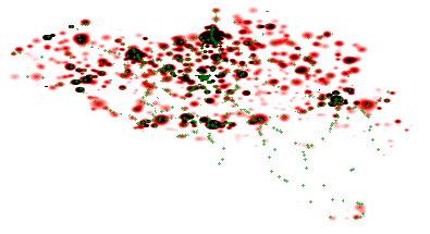
Fig. 4: Heatmap of the population distribution in Belgium, which is illustrated for each cell as a scale going from white (low), to red (medium) and black (high). The actual placement of train stops are indicated as green points.
Stops
Stop generation is divided into two steps. First, stops are placed based on population values, then the edge generation step is initiated after which the second phase of stop generation is executed where additional stops are created based on the generated edges.
Population-based For the initial placement of stops, our algorithm only takes a population distribution as input. The algorithm iteratively selects random cells in the two-dimensional area, and tags those cells as stops. To make it region-based [21], the selection uses a weighted Zipf-like-distribution, where cells with high population values have a higher chance of being picked than cells with lower values. The shape of this Zipf curve can be scaled to allow for different stop distributions to be configured. Furthermore, a minimum distance between stops can be configured, to avoid situations where all stops are placed in highly populated areas.
Edge-based Another stop generation phase exists after the edge generation because real transit networks typically show line artifacts for stop placement. Subfig. 5.1 shows the actual train stops in Belgium, which clearly shows line structures. Stop placement after the first generation phase results can be seen in Subfig. 5.2, which does not show these line structures. After the second stop generation phase, these line structures become more apparent as can be seen in Subfig. 5.3.

Subfig. 5.1: Real stops with line structures.
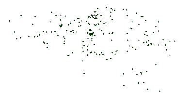
Subfig. 5.2: Synthetic stops after the first stop generation phase without line structures.
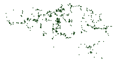
Subfig. 5.3: Synthetic stops after the second stop generation phase with line structures.
Fig. 5: Placement of train stops in Belgium, each dot represents one stop.
In this second stop generation phase, edges are modified so that sufficiently populated areas will be included in paths formed by edges, as illustrated by Fig. 6. Random edges will iteratively be selected, weighted by the edge length measured as Euclidian distance. (The Euclidian distance based on geographical coordinates is always used to calculate distances in this work.) On each edge, a random cell is selected weighed by the population value in the cell. Next, a weighed random point in a certain area around this point is selected. This selected point is marked as a stop, the original edge is removed and two new edges are added, marking the path between the two original edge nodes and the newly selected node.

Subfig. 6.1: Selecting a weighted random point on the edge.

Subfig. 6.2: Defining an area around the selected point.

Subfig. 6.3: Choosing a random point within the area, weighted by population value.

Subfig. 6.4: Modify edges so that the path includes this new point.
Fig. 6: Illustration of the second phase of stop generation where edges are modified to include sufficiently populated areas in paths.
Edges
The next phase in public transit network generation connects stops that were generated in the previous phase with edges. In order to simulate real transit network structures, we split up this generation phase into three sequential steps. In the first step, clusters of nearby stops are formed, to lay the foundation for short-distance routes. Next, these local clusters are connected with each other, to be able to form long-distance routes. Finally, a cleanup step is in place to avoid abnormal edge structures in the network.
Short-distance The formation of clusters with nearby stations is done using agglomerative hierarchical clustering. Initially, each stop is part of a seperate cluster, where each cluster always maintains its centroid. The clustering step will iteratively try to merge two clusters with their centroid distance below a certain threshold. This threshold will increase for each iteration, until a maximum value is reached. The maximum distance value indicates the maximum inter-stop distance for forming local clusters. When merging two clusters, an edge is added between the closest stations from the respective clusters. The center location of the new cluster is also recalculated before the next iteration.
Long-distance At this stage, we have several clusters of nearby stops. Because all stops need to be reachable from all stops, these separate clusters also need to be connected. This problem is related to the domain of route planning over public transit networks, in which networks can be decomposed into smaller clusters of nearby stations to improve the efficiency of route planning. Each cluster contains one or more border stations [27], which are the only points through which routes can be formed between different clusters. We reuse this concept of border stations, by iteratively picking a random cluster, identifying its closest cluster based on the minimal possible stop distance, and connecting their border stations using a new edge. After that, the two clusters are merged. The iteration will halt when all clusters are merged and there is only one connected graph.
Cleanup The final cleanup step will make sure that the number of stops that are connected by only one edge are reduced. In real train networks, the majority of stations are connected with at least more than one other station. The two earlier generation steps however generate a significant number of loose stops, which are connected with only a single other stop with a direct edge. In this step, these loose stops are identified, and an attempt is made to connect them to other nearby stops as shown in Algorithm 1. For each loose stop, this is done by first identifying the direction of the single edge of the loose stop on line 18. This direction is scaled by the radius in which to look for stops, and defines the stepsize for the loop that starts on line 20. This loop starts from the loose stop and iteratively moves the search position in the defined direction, until it finds a random stop in the radius, or the search distance exceeds the average distance between the stops in the neighbourhood of this loose stop. This random stop from line 22 can be determined by finding all stations that have a distance to the search point that is below the radius, and picking a random stop from this collection. If such a stop is found, an edge is added from our loose stop to this stop.
FUNCTION RemoveLooseStops(S, E, N, O, r)INPUT:Set of stops SSet of edges E between the stops from SMaximum number N of closest stations to considerMaximum average distance O around a stop to be considereda loose stationRadius r in which to look for stops.FOREACH s in S with degree of 1 w.r.t. E DOsx = x coordinate of ssy = y coordinate of sC = N closest stations to s in S excluding sc = closest station to s in S excluding scx = x coordinate of ccy = y coordinate of ca = average distance between each pair of stops in CIF a <= O and C not empty THENdx= (sx - cx) * rdy= (sy - cy) * rox = sx; oy = syWHILE distance between o and s < a DOox += dx; oy += dys' = random station around o with radius a * rIF s' existsadd edge between s and s' to E and continuenext for-loop iteration
Algorithm 1: Reduce the number of loose stops by adding additional edges.
Fig. 7 shows an example of these three steps. After this phase, a network with stops and edges is available, and the actual transit planning can commence.

Subfig. 7.1: Formation of local clusters.

Subfig. 7.2: Connecting clusters through border stations.

Subfig. 7.3: Cleanup of loose stops.
Fig. 7: Example of the different steps in the edges generation algorithm.
Generator Objectives The main guaranteed objective of the edge generator is that the stops form a single connected transit network graph. This is to ensure that all stops in the network can be reached from any other stop using at least one path through the network.
Routes
Given a network of stops and edges, this phase generates routes over the network. This is done by creating short and long distance routes in two sequential steps.
Short-distance The goal of the first step is to create short routes where vehicles deliver each passed stop. This step makes sure that all edges are used in at least one route, this ensures that each stop can at least be reached from each other stop with one or more transfers to another line. The algorithm does this by first determining a subset of the largest stops in the network, based on the population value. The shortest path from each large stop to each other large stop through the network is determined. if this shortest path is shorter than a predetermined value in terms of the number of edges, then this path is stored as a route, in which all passed stops are considered as actual stops in the route. For each edge that has not yet been passed after this, a route is created by iteratively adding unpassed edges to the route that are connected to the edge until an edge is found that has already been passed.
Long-distance In the next step, longer routes are created, where the transport vehicle not necessarily halts at each passed stop. This is done by iteratively picking two stops from the list of largest stops using the network-based method [21] with each stop having an equal chance to be selected. A heuristical shortest path algorithm is used to determine a route between these stops. This algorithm searches for edges in the geographical direction of the target stop. This is done to limit the complexity of finding long paths through potentially large networks. A random amount of the largest stops on the path are selected, where the amount is a value between a minimum and maximum preconfigured route length. This iteration ends when a predetermined number of routes are generated.
Generator Objectives This algorithm takes into account the objectives of route design [19], as discussed in Section 2.2. More specifically, by first focusing on the largest stops, a minimal level of area coverage and demand satisfaction is achieved, because the largest stops correspond to highly populated areas, which therefore satisfies at least a large part of the population. By determining the shortest path between these largest stops, the route and trip directness between these stops is optimal. Finally, by not instantiating all possible routes over the network, the total route length is limited to a reasonable level.
Trips
A time-agnostic transit network with routes has been generated in the previous steps. In this final phase, we temporally instantiate routes by first determining starting times for trips, after which the following stop times can be calculated based on route distances. Instead of generating explicit timetables, as is done in typical transit scheduling methodologies, we create fictional rides of vehicles. In order to achieve realistic trip times, we approximate real trip time distributions, with the possibility to encounter delays.
As mentioned before in Section 2.2, each consecutive pair of start and stop time in a trip over an edge corresponds to a connection. A connection can therefore be represented as a pair of timestamps, a link to the edge representing the departure and arrival stop, a link to the trip it is part of, and its index within this trip.
Trip Starting Times The trips generator iteratively creates new connections until a predefined number is reached. For each connection, a random route is selected with a larger chance of picking a long route. Next, a random start time of the connection is determined. This is done by first picking a random day within a certain range. After that, a random hour of the day is determined using a preconfigured distribution. This distribution is derived from the public logs of iRail, a route planning API in Belgium [28]. A seperate hourly distribution is used for weekdays and weekends, which is chosen depending on the random day that was determined.
Stop Times Once the route and the starting time have been determined, different stop times across the trip can be calculated. For this, we take into account the following factors:
- Maximum vehicle speed , preconfigured constant.
- Vehicle acceleration , preconfigured constant.
- Connection distance , Euclidian distance between stops in network.
- Stop size , derived from population value.
For each connection in the trip, the time it takes for a vehicle to move between the two stops over a certain distance is calculated using the formula in Equation 3. Equation 1 calculates the required time to reach maximum speed and Equation 2 calculates the required distance to reach maximum speed. This formula simulates the vehicle speeding up until its maximum speed, and slowing down again until it reaches its destination. When the distance is too short, the vehicle will not reach its maximum speed, and just speeds up as long as possible until is has to slow down again to stop in time.
Equation 1: Time to reach maximum speed.
Equation 2: Distance to reach maximum speed.
Equation 3: Duration for a vehicle to move between two stops.
Not only the connection duration, but also the waiting times of the vehicle at each stop are important for determining the stop times. These are calculated as a constant minimum waiting time together with a waiting time that increases for larger stop sizes , this increase is determined by a predefined growth factor.
Delays Finally, each connection in the trip will have a certain chance to encounter a delay. When a delay is applicable, a delay value is randomly chosen within a certain range. Next to this, also a cause of the delay is determined from a preconfigured list. These causes are based on the Traffic Element Events from the Transport Disruption ontology, which contains a number of events that are not planned by the network operator such as strikes, bad weather or animal collisions. Different types of delays can have a different impact factor of the delay value, for instance, simple delays caused by rush hour would have a lower impact factor than a major train defect. Delays are carried over to next connections in the trip, with again a chance of encountering additional delay. Furthermore, these delay values can also be reduced when carried over to the next connection by a certain predetermined factor, which simulates the attempt to reduce delays by letting vehicles drive faster.
Generator Objectives For trip generation, we take into account several objectives from the setting of frequencies and timetabling from transit planning [19]. By instantiating more long distance routes, we aim to increase demand satisfaction as much as possible, because these routes deliver busy and populated areas, and the goal is to deliver these more frequently. Furthermore, by taking into account realistic time distributions for trip instantiation, we also adhere to this objective. Secondly, by ensuring waiting times at each stop that are longer for larger stations, the transfer coordination objective is taken into account to some extent.
Implementation
In this section, we discuss the implementation details of PoDiGG, based on the generator algorithm introduced in Section 2.5. PoDiGG is split up into two parts: the main PoDiGG generator, which outputs GTFS data, and PoDiGG-LC, which depends on the main generator to output RDF data. Serialization in RDF using existing ontologies, such as the GTFS and Linked Connections ontologies, allows this inherently linked data to be used within RDF data management systems, where it can for instance be used for benchmarking purposes. Providing output in GTFS will allow this data to be used directly within all systems that are able to handle transit feeds, such as route planning systems. The two generator parts will be explained hereafter, followed by a section on how the generator can be configured using various parameters.
PoDiGG
The main requirement of our system is the ability to generate realistic public transport datasets using the mimicking algorithm that was introduced in Section 2.5. This means that given a population distribution of a certain region, the system must be able to design a network of routes, and determine timely trips over this network.
PoDiGG is implemented to achieve this goal. It is written in JavaScript using Node.js, and is available under an open license on GitHub. In order to make installation and usage more convenient, PoDiGG is available as a Node module on the NPM package manager and as a Docker image on Docker Hub to easily run on any platform. Every sub-generator that was explained in Section 2.5, is implemented as a separate module. This makes PoDiGG highly modifiable and composable, because different implementations of sub-generators can easily be added and removed. Furthermore, this flexible composition makes it possible to use real data instead of certain sub-generators. This can be useful for instance when a certain public transport network is already available, and only the trips and connections need to be generated.
We designed PoDiGG to be highly configurable to adjust the characteristics of the generated output across different levels, and to define a certain seed parameter for producing deterministic output.
All sub-generators store generated data in-memory, using list-based data structures directly corresponding to the GTFS format.
This makes GTFS serialization a simple and efficient process.
Table 1 shows the GTFS files that are generated by the different PoDiGG modules.
This table does not contain references to the region and edges generator,
because they are only used internally as prerequisites to the later steps.
All required files are created to have a valid GTFS dataset.
Next to that, the optional file for exceptional service dates is created.
Furthermore, delays.txt is created, which is not part of the GTFS specification.
It is an extension we provide in order to serialize delay information about each connection in a trip.
These delays are represented in a CSV file containing columns for referring to a connection in a trip,
and contains delay values in milliseconds and a certain reason per connection arrival and departure,
as shown in Listing 2.
| File | Generator |
|---|---|
agency.txt |
Constant |
stops.txt |
Stops |
routes.txt |
Routes |
trips.txt |
Trips |
stop_times.txt |
Trips |
calendar.txt |
Trips |
calendar_dates.txt |
Trips |
delays.txt |
Trips |
Table 1: The GTFS files that are written by PoDiGG, with their corresponding sub-generators that are responsible for generating the required data. The files in bold refer to files that are required by the GTFS specification.
trip_id,stop,delay_dep,delay_arr,delay_dep_reason,delay_arr_reason100_4 ,0 ,0 ,1405754 , ,td:RepairWork100_6 ,0 ,0 ,1751671 , ,td:BrokenTrain100_6 ,1 ,1751671 ,1553820 ,td:BrokenTrain ,td:BrokenTrain100_7 ,0 ,2782295 ,0 ,td:TreeWork ,
Listing 2: Sample of a delays.txt file in a GTFS dataset.
In order to easily observe the network structure in the generated datasets, PoDiGG will always produce a figure accompanying the GTFS dataset. Fig. 8 shows an example of such a visualization.
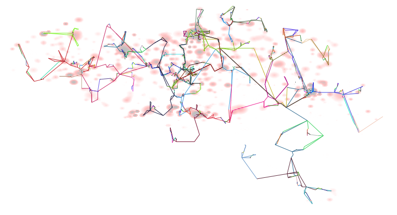
Fig. 8: Visualization of a generated public transport network based on Belgium’s population distribution. Each route has a different color, and dark route colors indicate more frequent trips over them than light colors. The population distribution is illustrated for each cell as a scale going from white (low), to red (medium) and black (high). Full image
Because the generation of large datasets can take a long time depending on the used parameters, PoDiGG has a logging mechanism, which provides continuous feedback to the user about the current status and progress of the generator.
Finally, PoDiGG provides the option to derive realistic public transit queries over the generated network, aimed at testing the load of route planning systems. This is done by iteratively selecting two random stops weighed by their size and choosing a random starting time based on the same time distribution as discussed in Subsection 2.5.5. This is serialized to a JSON format that was introduced for benchmarking the Linked Connections route planner [11].
PoDiGG-LC
PoDiGG-LC is an extension of PoDiGG, that outputs data in Turtle/RDF using the ontologies shown in Fig. 3. It is also implemented in JavaScript using Node.js, and available under an open license on GitHub. PoDiGG-LC is also available as a Node module on NPM and as a Docker image on Docker Hub. For this, we extended the GTFS-LC tool that is able to convert GTFS datasets to RDF using the Linked Connections and GTFS ontologies. The original tool serializes a minimal subset of the GTFS data, aimed at being used for Linked Connections route planning over connections. Our extension also serializes trip, station and route instances, with their relevant interlinking. Furthermore, our GTFS extension for representing delays is also supported, and is serialized using a new Linked Connections Delay ontology that we created.
Configuration
PoDiGG accepts a wide range of parameters that can be used to configure properties of the different sub-generators. Table 2 shows an overview of the parameters, grouped by each sub-generator. PoDiGG and PoDiGG-LC accept these parameters either in a JSON configuration file or via environment variables. Both PoDiGG and PoDiGG-LC produce deterministic output for identical sets of parameters, so that datasets can easily be reproduced given the configuration. The seed parameter can be used to introduce pseudo-randomness into the output.
| Name | Default Value | Description | |
|---|---|---|---|
seed |
1 |
The random seed | |
| Region | region_generator |
isolated |
Name of a region generator. (isolated, noisy or region) |
lat_offset |
0 |
Value to add with all generated latitudes | |
lon_offset |
0 |
Value to add with all generated longitudes | |
cells_per_latlon |
100 |
How many cells go in 1 latitude/longitude | |
| Stops | stops |
600 |
How many stops should be generated |
min_station_size |
0.01 |
Minimum cell population value for a stop to form | |
max_station_size |
30 |
Maximum cell population value for a stop to form | |
start_stop_choice_power |
4 |
Power for selecting large population cells as stops | |
min_interstop_distance |
1 |
Minimum distance between stops in number of cells | |
factor_stops_post_edges |
0.66 |
Factor of stops to generate after edges | |
edge_choice_power |
2 |
Power for selecting longer edges to generate stops on | |
stop_around_edge_choice_power |
4 |
Power for selecting large population cells around edges | |
stop_around_edge_radius |
2 |
Radius in number of cells around an edge to select points | |
| Edges | max_intracluster_distance |
100 |
Maximum distance between stops in one cluster |
max_intracluster_distance_growthfactor |
0.1 |
Power for clustering with more distant stops | |
post_cluster_max_intracluster_distancefactor |
1.5 |
Power for connecting a stop with multiple stops | |
loosestations_neighbourcount |
3 |
Neighbours around a loose station that should define its area | |
loosestations_max_range_factor |
0.3 |
Maximum loose station range relative to the total region size | |
loosestations_max_iterations |
10 |
Maximum iteration number to try to connect one loose station | |
loosestations_search_radius_factor |
0.5 |
Loose station neighbourhood size factor | |
| Routes | routes |
1000 |
The number of routes to generate |
largest_stations_fraction |
0.05 |
The fraction of stops to form routes between | |
penalize_station_size_area |
10 |
The area in which stop sizes should be penalized | |
max_route_length |
10 |
Maximum number of edges for a route in the macro-step | |
min_route_length |
4 |
Minimum number of edges for a route in the macro-step | |
| Connections | time_initial |
0 |
The initial timestamp (ms) |
time_final |
24 * 3600000 |
The final timestamp (ms) | |
connections |
30000 |
Number of connections to generate | |
stop_wait_min |
60000 |
Minimum waiting time per stop | |
stop_wait_size_factor |
60000 |
Waiting time to add multiplied by station size | |
route_choice_power |
2 |
Power for selecting longer routes for connections | |
vehicle_max_speed |
160 |
Maximum speed of a vehicle in km/h | |
vehicle_speedup |
1000 |
Vehicle speedup in km/(h2) | |
hourly_weekday_distribution |
...1 |
Hourly connection chances for weekdays | |
hourly_weekend_distribution |
...1 |
Hourly connection chances for weekend days | |
delay_chance |
0 |
Chance for a connection delay | |
delay_max |
3600000 |
Maximum delay | |
delay_choice_power |
1 |
Power for selecting larger delays | |
delay_reasons |
...2 |
Default reasons and chances for delays | |
delay_reduction_duration_fraction |
0.1 |
Maximum part of connection duration to subtract for delays | |
| Queryset | start_stop_choice_power |
4 |
Power for selecting large starting stations |
query_count |
100 |
The number of queries to generate | |
time_initial |
0 |
The initial timestamp | |
time_final |
24 * 3600000 |
The final timestamp | |
max_time_before_departure |
3600000 |
Minimum number of edges for a route in the macro-step | |
hourly_weekday_distribution |
...1 |
Chance for each hour to have a connection on a weekday | |
hourly_weekend_distribution |
...1 |
Chance for each hour to have a connection on a weekend day |
Table 2: Configuration parameters for the different sub-generators. Time values are represented in milliseconds. 1 Time distributions are based on public route planning logs [28]. 2 Default delays are based on the Transport Disruption ontology.
Evaluation
In this section, we discuss our evaluation of PoDiGG. We first evaluate the realism of the generated datasets using a constant seed by comparing its coherence to real datasets, followed by a more detailed realism evaluation of each sub-generator using distance functions. Finally, we provide an indicative efficiency and scalability evaluation of the generator and discuss practical dataset sizes. All scripts that were used for the following evaluation can be found on GitHub. Our experiments were executed on a 64-bit Ubuntu 14.04 machine with 128 GB of memory and a 24-core 2.40 GHz CPU.
Coherence
Metric
In order to determine how closely synthetic RDF datasets resemble their real-world variants in terms of structuredness, the coherence metric [10] can be used. In RDF dataset generation, the goal is to reach a level of structuredness similar to real datasets. As mentioned before in Section 2.2, many synthetic datasets have a level of structuredness that is higher than their real-world counterparts. Therefore, our coherence evaluation should indicate that our generator is not subject to the same problem. We have implemented a command-line tool to calculate the coherence value for any given input dataset.
Results
When measuring the coherence of the Belgian railway, buses and Dutch railway datasets, we discover high values for both the real-world datasets and the synthetic datasets, as can be seen in Table 3. These nearly maximal values indicate that there is a very high level of structuredness in these real-world datasets. Most instances have all the possible values, unlike most typical RDF datasets, which have values around or below 0.6 [10]. That is because of the very specialized nature of this dataset, and the fact that they originate from GTFS datasets that have the characteristics of relational databases. Only a very limited number of classes and predicates are used, where almost all instances have the same set of attributes. In fact, these very high coherence values for real-world datasets simplify the process of synthetic dataset generation, as less attention needs to be given to factors that lead to lower levels of structuredness, such as optional attributes for instances. When generating synthetic datasets using PoDiGG with the same number of stops, routes and connections for the three gold standards, we measure very similar coherence values, with differences ranging from 0.08% to 1.64%. This confirms that PoDiGG is able to create datasets with the same high level of structuredness to real datasets of these types, as it inherits the relational database characteristics from its GTFS-centric mimicking algorithm.
| Belgian railway | Belgian buses | Dutch railway | |
|---|---|---|---|
| Real | 0.9845 | 0.9969 | 0.9862 |
| Synthetic | 0.9879 | 0.9805 | 0.9870 |
| Difference | 0.0034 | 0.0164 | 0.0008 |
Table 3: Coherence values for three gold standards compared to the values for equivalent synthetic variants.
Distance to Gold Standards
While the coherence metric is useful to compare the level of structuredness between datasets, it does not give any detailed information about how real synthetic datasets are in terms of their distance to the real datasets. In this case, we are working with public transit feeds with a known structure, so we can look at the different datasets aspects in more detail. More specifically, we start from real geographical areas with their population distributions, and consider the distance functions between stops, edges, routes and trips for the synthetic and gold standard datasets. In order to check the applicability of PoDiGG to different transport types and geographical areas, we compare with the gold standard data of the Belgian railway, the Belgian buses and the Dutch railway. The scripts that were used to derive these gold standards from real-world data can be found on GitHub.
In order to construct distance functions for the different generator elements, we consider several helper functions. The function in Equation 4 is used to determine the closest element in a set of elements to a given element , given a distance function . The function in Equation 5 calculates the distance between all elements in and all elements in , given a distance function . The computational complexity of is , where is the cost for one distance calculation for . The complexity of then becomes .
Equation 4: Function to determine the closest element in a set of elements.
Equation 5: Function to calculate the distance between all elements in a set of elements.
Stops Distance
For measuring the distance between two sets of stops and , we introduce the distance function from Equation 6. This measures the distance between every possible pair of stops using the Euclidean distance function . Assuming a constant execution time for , the computational complexity for is .
Equation 6: Function to calculate the distance between two sets of stops.
Edges Distance
In order to measure the distance between two sets of edges and , we use the distance function from Equation 7, which measures the distance between all pairs of edges using the distance function . This distance function , which is introduced in Equation 8, measures the Euclidean distance between the start and endpoints of each edge, and between the different edges, weighed by the length of the edges. The constant in Equation 8 is to ensure that the distance between two edges that have an equal length, but exist at a different position, is not necessarily zero. The computational cost of can be considered as a constant, so the complexity of becomes .
Equation 7: Function to calculate the distance between two sets of edges.
Equation 8: Function to calculate the distance between two edges.
Routes Distance
Similarly, the distance between two sets of routes and is measured in Equation 9 by applying for the distance function . Equation 10 introduces this distance function between two routes, which is calculated by considering the edges in each route and measuring the distance between those two sets using the distance function from Equation 7. By considering the maximum amount of edges per route as , the complexity of becomes This leads to a complexity of for .
Equation 9: Function to calculate the distance between two sets of routes.
Equation 10: Function to calculate the distance between two routes.
Connections Distance
Finally, we measure the distance between two sets of connections and using the function from Equation 11. The distance between two connections is measured using the function from Equation 12, which is done by considering their respective temporal distance weighed by a constant –when serializing time in milliseconds, we set to –, and their geospatial distance using the edge distance function . The complexity of time calculation in can be considered being constant, which makes it overall complexity . For , this leads to a complexity of .
Equation 11: Function to calculate the distance between two sets of connections.
Equation 12: Function to calculate the distance between two connections.
Computability
When using the introduced functions for calculating the distance between stops, edges, routes or connections, execution times can become long for a large number of elements because of their large complexity. When applying these distance functions for realistic numbers of stops, edges, routes and connections, several optimizations should be done in order to calculate these distances in a reasonable time. A major contributor for these high complexities is for finding the closest element from a set of elements to a given element, as introduced in Equation 4. In practice, we only observed extreme execution times for the respective distance between routes and connections. For routes, we implemented an optimization, with the same worst-case complexity, that indexes routes based on their geospatial position, and performs radial search around each route when the closest one from a set of other routes should be found. For connections, we consider the linear time dimension when performing binary search for finding the closest connection within a set of elements.
Metrics
In order to measure the realism of each generator phase, we introduce a realism factor for each phase. These values are calculated by measuring the distance from randomly generated elements to the gold standard, divided by the distance from the actually generated elements to the gold standard, as shown below for respectively stops, edges, routes and connections. We consider these randomly generated elements having the lowest possible level of realism, so we use these as a weighting factor in our realism values.
Results
We measured these realism values with gold standards for the Belgian railway, the Belgian buses and the Dutch railway. In each case, we used an optimal set of parameters to achieve the most realistic generated output. Table 4 shows the realism values for the three cases, which are visualized in Fig. 9, Fig. 10, Fig. 11 and Fig. 12. Each value is larger than 1, showing that the generator at least produces data that is closer to the gold standard, and is therefore more realistic. The realism for edges is in each case very large, showing that our algorithm produces edges that are very similar to actual the edge placement in public transport networks according to our distance function. Next, the realism of stops is lower, but still sufficiently high to consider it as realistic. Finally, the values for routes and connections show that these sub-generators produce output that is closer to the gold standard than the random function according to our distance function. Routes achieve the best level of realism for the Belgian railway case. For this same case, the connections are however only slightly closer to the gold standard than random placement, while for the other cases the realism is more significant. All of these realism values show that PoDiGG is able to produce realistic data for different regions and different transport types.
| Belgian railway | Belgian buses | Dutch railway | |
|---|---|---|---|
| Stops | 5.5490 | 297.0888 | 4.0017 |
| Edges | 147.4209 | 1633.4693 | 318.4131 |
| Routes | 2.2420 | 0.0164 | 1.3095 |
| Connections | 1.0451 | 1.5006 | 1.3017 |
Table 4: Realism values for the three gold standards in case of the different sub-generators, respectively calculated for the stops , edges , routes and connections .
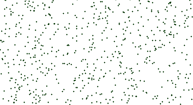
Subfig. 9.1: Random

Subfig. 9.2: Generated
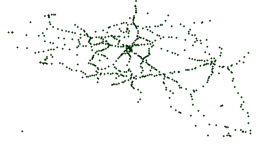
Subfig. 9.3: Gold standard
Fig. 9: Stops for the Belgian railway case.
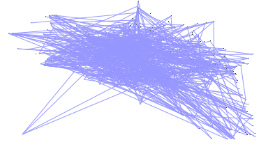
Subfig. 10.1: Random
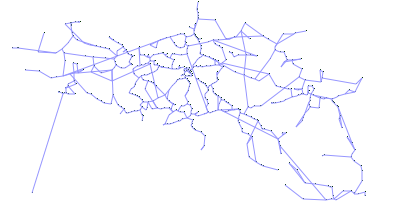
Subfig. 10.2: Generated
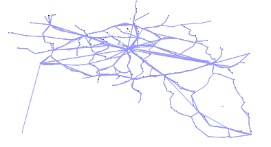
Subfig. 10.3: Gold standard
Fig. 10: Edges for the Belgian railway case.
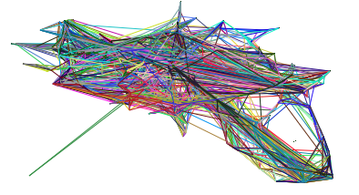
Subfig. 11.1: Random

Subfig. 11.2: Generated
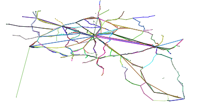
Subfig. 11.3: Gold standard
Fig. 11: Routes for the Belgian railway case.

Fig. 12: Connections per hour for the Belgian railway case.
Performance
Metrics
While performance is not the main focus of this work, we provide an indicative performance evaluation in this section in order to discover the bottlenecks and limitations of our current implementation that could be further investigated and resolved in future work. We measure the impact of different parameters on the execution times of the generator. The three main parameters for increasing the output dataset size are the number of stops, routes and connections. Because the number of edges is implicitly derived from the number of stops in order to reach a connected network, this can not be configured directly. In this section, we start from a set of parameters that produces realistic output data that is similar to the Belgian railway case. We let the value for each of these parameters increase to see the evolution of the execution times and memory usage.
Results
Fig. 13 shows a linear increase in execution times when increasing the routes or connections. The execution times for stops do however increase much faster, which is caused by the higher complexity of networks that are formed for many stops. The used algorithms for producing this network graph proves to be the main bottleneck when generating large networks. Networks with a limited size can however be generated quickly, for any number of routes and connections. The memory usage results from Fig. 14 also show a linear increase, but now the increase for routes and connections is higher than for the stops parameter. These figures show that stops generation is a more CPU intensive process than routes and connections generation. These last two are able to make better usage of the available memory for speeding up the process.

Fig. 13: Execution times when increasing the number of stops, routes or connections.

Fig. 14: Memory usage when increasing the number of stops, routes or connections.
Dataset size
An important aspect of dataset generation is its ability to output various dataset sizes. In PoDiGG, different options are available for tweaking these sizes. Increasing the time range parameter within the generator increases the number of connections while the number of stops and routes will remain the same. When enlarging the geographical area over the same period of time, the opposite is true. As a rule of thumb, based on the number of triples per connection, stops and routes, the total number of generated triples per dataset is approximately . For the Belgian railway case, containing 30,011 connections over a period of 9 months, with 583 stops and 362 routes, this would theoretically result in 213,937 triples. In practice, we reach 235,700 triples when running with these parameters, which is slightly higher because of the other triples that are not taken into account for this simplified formula, such as the ones for trips, stations and delays.
Discussion
In this section, we discuss the main characteristics, the usage within benchmarks and the limitations of this work. Finally, we mention several PoDiGG use cases.
Characteristics
Our main research question on how to generate realistic synthetic public transport networks has been answered by the introduction of the mimicking algorithm from Section 2.5, based on commonly used practises in transit network design. This is based on the accepted hypothesis that the population distribution of an area is correlated with its transport network design and scheduling. We measured the realism of the generated datasets using the coherence metric in Subsection 2.7.1 and more fine-grained realism metrics for different public transport aspects in Subsection 2.7.2.
PoDiGG, our implementation of the algorithm, accepts a wide range of parameters to configure the mimicking algorithm. PoDiGG and PoDiGG-LC are able to output the mimicked data respectively as GTFS and RDF datasets, together with a visualization of the generated transit network. Our system can be used without requiring any extensive setup or advanced programming skills, as it consists of simple command lines tools that can be invoked with a number of optional parameters to configure the generator. Our system is proven to be generalizable to other transport types, as we evaluated PoDiGG for the bus and train transport type, and the Belgium and Netherlands geospatial regions in Subsection 2.7.2.
Usage within Benchmarks
A synthetic dataset generator, which is one of the main contributions of this work, forms an essential aspect of benchmarks for (RDF) data management systems [23, 29]. Prescribing a concrete benchmark that includes the evaluation of tasks is out of scope. However, to provide a guideline on how our dataset generator can be used as part of a benchmark, we relate the primary elements of public transport datasets to choke points in data management systems, i.e., key technical challenges in these systems. Below, we list choke points related to storage and querying within data management systems and route planning systems. For each choke point, we introduce example tasks to evaluate them in the context of public transport datasets. The querying choke points are inspired by the choke points identified by Petzka et. al. for faceted browsing [30].
- Storage of entities.
- Storage of stops, stations, connections, routes, trips and delays.
- Storage of links between entities.
- Storage of stops per station.
- Storage of connections for stops.
- Storage of the next connection for each connection.
- Storage of connections per trip.
- Storage of trips per route.
- Storage of a connection per delay.
- Storage of literals.
- Storage of latitude, longitude, platform code and code of stops.
- Storage of latitude, longitude and label of stations.
- Storage of delay durations.
- Storage of the start and end time of connections.
- Storage of sequences.
- Storage of sequences of connections.
- Find instances by property value.
- Find latitude, longitude, platform code or code by stop.
- Find station by stop.
- Find country by station.
- Find latitude, longitude, or label by station.
- Find delay by connection.
- Find next connection by connection.
- Find trip by connection.
- Find route by connection.
- Find route by trip.
- Find instances by inverse property value.
- Inverse of examples above.
- Find instances by a combination of properties values.
- Find stops by geospatial location.
- Find stations by geospatial location.
- Find instances for a certain property path with a certain value.
- Find the delay value of the connection after a given connection.
- Find the delay values of all connections after a given connection.
- Find instances by inverse property path with a certain value.
- Find stops that are part of a certain trip that passes by the stop at the given geospatial location.
- Find instances by class, including subclasses.
- Find delays of a certain class.
- Find instances with a numerical value within a certain interval.
- Find stops by latitude or longitude range.
- Find stations by latitude or longitude range.
- Find delays with durations within a certain range.
- Find instances with a combination of numerical values within a certain interval.
- Find stops by geospatial range.
- Find stations by geospatial range.
- Find instances with a numerical interval by a certain value for a certain property path.
- Find connections that pass by stops in a given geospatial range.
- Find instances with a numerical interval by a certain value.
- Find connections that occur at a certain time.
- Find instances with a numerical interval by a certain value for a certain property path.
- Find trips that occur at a certain time.
- Find instances with a numerical interval by a certain interval.
- Find connections that occur during a certain time interval.
- Find instances with a numerical interval by a certain interval for a certain property path.
- Find trips that occur during a certain time interval.
- Find instances with numerical intervals by intervals with property paths.
- Find connections that occur during a certain time interval with stations that have stops in a given geospatial range.
- Find trips that occur during a certain time interval with stops in a given geospatial range.
- Plan a route that gets me from stop A to stop B starting at a certain time.
This list of choke points and tasks can be used as a basis for benchmarking spatiotemporal data management systems using public transport datasets. For example, SPARQL queries can be developed based on these tasks and executed by systems using a public transport dataset. For the benchmarking with these tasks, it is essential that the used datasets are realistic, as discussed in Subsection 2.7.2. Otherwise, certain choke points may not resemble the real world. For example, if an unrealistic dataset would contain only a single trip that goes over all stops, then finding a route between two given stops could be unrealistically simple.
Limitations and Future Work
In this section, we discuss the limitations of the current mimicking algorithm and its implementation, together with further research opportunities.
Memory Usage
The sequential steps in the presented mimicking algorithm require persistence of the intermediary data that is generated in each step. Currently, PoDiGG is implemented in such a way that all data is kept in-memory for the duration of the generation, until it is serialized. When large datasets need to be generated, this requires a larger amount of memory to be allocated to the generator. Especially for large amounts of routes or connections, where 100 million connections already require almost 10GB of memory to be allocated. While performance was not the primary concern in this work, in future work, improvements could be made. A first possible solution would be to use a memory-mapped database for intermediary data, so that not all data must remain in memory at all times. An alternative solution would be to modify the mimicking process to a streaming algorithm, so that only small parts of data need to be kept in memory for datasets of any size. Considering the complexity of transit networks, a pure streaming algorithm might not be feasible, because route design requires knowledge of the whole network. The generation of connections however, could be adapted so that it works as a streaming algorithm.
Realism
We aimed to produce realistic transit feeds by reusing the methodologies learned in public transit planning. Our current evaluation compares generated output to real datasets, as no similar generators currently exist. When similar generation algorithms are introduced in the future, this evaluation can be extended to compare their levels of realism. Our results showed that all sub-generators, except for the trips generator, produced output with a high realism value. The trips are still closer to real data than a random generator, but this can be further improved in future work. This can be done by for instance taking into account network capacities [19] on certain edges when instantiating routes as trips. This is because we currently assume infinite edge capacities, which can result in a large amount of connections over an edge at the same time, which may not be realistic for certain networks. Alternatively, we could include other factors in the generation algorithm, such as the location of certain points of interest, such as shopping areas, schools and tourist spots. In the future, a study could be done to identify and measure the impact of certain points of interest on transit networks, which could be used as additional input to the generation algorithm to further improve the level of realism. Next to this, in order to improve transfer coordination [19], possible transfers between trips should be taken into account when generating stop times. Limiting the network capacity will also lead to natural congestion of networks [21], which should also be taken into account for improving the realism. Furthermore, the total vehicle fleet size [19] should be considered, because we currently assume an infinite number of available vehicles. It is more realistic to have a limited availability of vehicles in a network, with the last position of each vehicle being of importance when choosing the next trip for that vehicle.
Alternative Implementations
An alternative way of implementing this generator would be to define declarative dependency rules for public transport networks, based on the work by Pengyue et. al. [22]. This would require a semantic extension to the engine so that it is aware of the relevant ontologies and that it can serialize to one or more RDF formats. Alternatively, machine learning techniques could be used to automatically learn the structure and characteristics of real datasets and create similar realistic synthetic datasets [31], or to create variants of existing datasets [32]. The downside of machine learning techniques is however that it is typically more difficult to tweak parameters of automatically learned models when specific characteristics of the output need to be changed, when compared to a manually implemented algorithm. Sensitivity analysis could help to determine the impact of such parameters in order to understand the learned models better.
Streaming Extension
Finally, the temporal aspect of public transport networks is useful for the domain of RDF stream processing [33]. Instead of producing single static datasets as output, PoDiGG could be adapted to produce RDF streams of connections and delays, where information about stops and routes are part of the background knowledge. Such an extension can become part of a benchmark, such as CityBench [34] and LSBench [18], for assessing the performance of RDF stream processing systems with temporal and geospatial capabilities.
PoDiGG In Use
PoDiGG and PoDiGG-LC have been developed for usage within the HOBBIT platform. This platform is being developed within the HOBBIT project and aims to provide an environment for benchmarking RDF systems for Big Linked Data. The platform provides several default dataset generators, including PoDiGG, which can be used to benchmark RDF systems.
PoDiGG, and its generated datasets are being used in the ESWC Mighty Storage Challenge 2017 and 2018 [35]. The first task of this challenge consists of RDF data ingestion into triple stores, and querying over this data. Because of the temporal aspect of public transport data in the form of connections, PoDiGG datasets are fragmented by connection departure time, and transformed to a data stream that can be inserted. In task 4 of this challenge, the efficiency of faceted browsing solutions is benchmarked [30]. In this work, a list of choke points are identified regarding SPARQL queries on triple stores, which includes points such as the selection of subclasses and property-path transitions. Because of the geographical property of public transport data, PoDiGG datasets are being used for this benchmark.
Finally, PoDiGG is being used for creating virtual transit networks of variable size for the purposes of benchmarking route planning frameworks, such as Linked Connections [11].
Conclusions
In this article, we introduced a mimicking algorithm for public transport data, based on steps that are used in real-world transit planning. Our method splits this process into several sub-generators and uses population distributions of an area as input. As part of this article, we introduced PoDiGG, a reusable framework that accepts a wide range of parameters to configure the generation algorithm.
Results show that the structuredness of generated datasets are similar to real public transport datasets. Furthermore, we introduced several functions for measuring the realism of synthetic public transport datasets compared to a gold standard on several levels, based on distance functions. The realism was confirmed for different regions and transport types. Finally, the execution times and memory usages were measured when increasing the most important parameters, which showed a linear increase for each parameter, showing that the generator is able to scale to large dataset outputs.
The public transport mimicking algorithm we introduced, with PoDiGG and PoDiGG-LC as implementations, is essential for properly benchmarking the efficiency and performance of public transport route planning systems under a wide range of realistic, but synthetic circumstances. Flexible configuration allows datasets of any size to be created and various characteristics to be tweaked to achieve highly specialized datasets for testing specific use cases. In general, our dataset generator can be used for the benchmarking of geospatial and temporal RDF data management systems, and therefore lowers the barrier towards more efficient and performant systems.
Storing Evolving Data
In this chapter, we tackle the second challenge of this PhD, which is: “Indexing evolving data involves a trade-off between storage size and lookup efficiency”. Since evolving knowledge graphs add a temporal dimension to regular knowledge graphs, new storage and querying techniques are required. A naive way to handle this temporal dimension would be to store each knowledge graph version as a separately materialized knowledge graph. This can however introduce a tremendous storage overhead when consecutive versions are similar to each other. Furthermore, querying over such a naive storage method would require going through all of these versions, which does not scale well with many versions.
The focus of our work in this chapter is to come up with a Web-friendly trade-off between storage size and lookup efficiency, so that evolving knowledge graphs can be published on the Web without requiring high-end machines. We introduce a new indexing technique for evolving data, that focuses on querying in a stream-based manner. This allows results to be sent to the client from the moment that they are found, which reduces waiting time compared to batch-based querying. Streaming is especially useful when the number of results is very large, and is memory friendly for machines with limited capabilities.
This chapter is based on the research question: “How can we store RDF archives to enable efficient versioned triple pattern queries with offsets?” We focus on triple pattern queries, as these are the fundamental building blocks for more complex SPARQL queries over knowledge graphs. For example, the Triple Pattern Fragments interface [36] exposes triple pattern access to datasets, which is sufficient for evaluating complex SPARQL queries on top of this. We answer our research question by introducing a storage technique that introduces various temporal indexes next to the typical indexes that are required for knowledge graphs. These indexes are essential for achieving efficient querying for different kinds of versioned queries. We extensively evaluate this approach based on our implementation OSTRICH. Our results show that our method achieves a trade-off between storage size and lookup efficiency that is useful for hosting evolving knowledge graphs on the Web. Concretely, at the cost of an increase in storage size and ingestion time, query execution time is significantly reduced. As storage is typically cheap, and ingestion can happen offline, this trade-off is acceptable in a Web environment.
Ruben Taelman, Miel Vander Sande, Joachim Van Herwegen, Erik Mannens, and Ruben Verborgh. 2019. Triple Storage for Random-Access Versioned Querying of RDF Archives. Journal of Web Semantics 54 (January 2019), 4–28.
Abstract
When publishing Linked Open Datasets on the Web, most attention is typically directed to their latest version. Nevertheless, useful information is present in or between previous versions. In order to exploit this historical information in dataset analysis, we can maintain history in RDF archives. Existing approaches either require much storage space, or they expose an insufficiently expressive or efficient interface with respect to querying demands. In this article, we introduce an RDF archive indexing technique that is able to store datasets with a low storage overhead, by compressing consecutive versions and adding metadata for reducing lookup times. We introduce algorithms based on this technique for efficiently evaluating queries at a certain version, between any two versions, and for versions. Using the BEAR RDF archiving benchmark, we evaluate our implementation, called OSTRICH. Results show that OSTRICH introduces a new trade-off regarding storage space, ingestion time, and querying efficiency. By processing and storing more metadata during ingestion time, it significantly lowers the average lookup time for versioning queries. OSTRICH performs better for many smaller dataset versions than for few larger dataset versions. Furthermore, it enables efficient offsets in query result streams, which facilitates random access in results. Our storage technique reduces query evaluation time for versioned queries through a preprocessing step during ingestion, which only in some cases increases storage space when compared to other approaches. This allows data owners to store and query multiple versions of their dataset efficiently, lowering the barrier to historical dataset publication and analysis.
Introduction
In the area of data analysis, there is an ongoing need for maintaining the history of datasets. Such archives can be used for looking up data at certain points in time, for requesting evolving changes, or for checking the temporal validity of these data [37]. With the continuously increasing number of Linked Open Datasets [5], archiving has become an issue for RDF [3] data as well. While the RDF data model itself is atemporal, Linked Datasets typically change over time [38] on dataset, schema, and/or instance level [39]. Such changes can include additions, modifications, or deletions of complete datasets, ontologies, and separate facts. While some evolving datasets, such as DBpedia [40], are published as separate dumps per version, more direct and efficient access to prior versions is desired.
Consequently, RDF archiving systems emerged that, for instance, support query engines that use the standard SPARQL query language [4]. In 2015, however, a survey on archiving Linked Open Data [37] illustrated the need for improved versioning capabilities, as current approaches have scalability issues at Web-scale. They either perform well for versioned query evaluation—at the cost of large storage space requirements—or require less storage space—at the cost of slower query evaluation. Furthermore, no existing solution performs well for all versioned query types, namely querying at, between, and for different versions. An efficient RDF archive solution should have a scalable storage model, efficient compression, and indexing methods that enable expressive versioned querying [37].
In this article, we argue that supporting both RDF archiving and SPARQL at once is difficult to scale due to their combined complexity. Instead, we propose an elementary but efficient versioned triple pattern index. Since triple patterns are the basic element of SPARQL, such indexes can serve as an entry point for query engines. Our solution is applicable as: (a) an alternative index with efficient triple-pattern-based access for existing engines, in order to improve the efficiency of more expressive SPARQL queries; and (b) a data source for the Web-friendly Triple Pattern Fragments [36] (TPF) interface, i.e., a Web API that provides access to RDF datasets by triple patterns and partitions the results in pages. We focus on the performance-critical features of stream-based results, query result offsets, and cardinality estimation. Stream-based results allow more memory-efficient processing when query results are plentiful. The capability to efficiently offset (and limit) a large stream reduces processing time if only a subset is needed. Cardinality estimation is essential for efficient query planning [36, 41] in many query engines.
Concretely, this work introduces a storage technique with the following contributions:
- a scalable versioned and compressed RDF index with offset support and result streaming;
- efficient query algorithms to evaluate triple pattern queries and perform cardinality estimation at, between, and for different versions, with optional offsets;
- an open-source implementation of this approach called OSTRICH;
- an extensive evaluation of OSTRICH compared to other approaches using an existing RDF archiving benchmark.
The main novelty of this work is the combination of efficient offset-enabled queries over a new index structure for RDF archives. We do not aim to compete with existing versioned SPARQL engines—full access to the language can instead be leveraged by different engines, or by using alternative RDF publication and querying methods such as the HTTP interface-based TPF approach. Optional versioning capabilities are possible for TPF by using VTPF [42], or datetime content-negotiation [43] through Memento [44].
This article is structured as follows. In the following section, we start by introducing the related work and our problem statement in Section 3.3. Next, in Section 3.4, we introduce the basic concepts of our approach, followed by our storage approach in Section 3.5, our ingestion algorithms in Section 3.6, and the accompanying querying algorithms in Section 3.7. After that, we present and discuss the evaluation of our implementation in Section 3.8. Finally, we present our conclusions in Section 3.9.
Related Work
In this section, we discuss existing solutions and techniques for indexing and compression in RDF storage, without archiving support. Then, we compare different RDF archiving solutions. Finally, we discuss suitable benchmarks and different query types for RDF archives. This section does not contain an exhaustive list of all relevant solutions and techniques, instead, only those that are most relevant to this work are mentioned.
General RDF Indexing and Compression
RDF storage systems typically use indexing and compression techniques for reducing query times and storage space. These systems can either be based on existing database technologies, such as relational databases [45] or document stores [46], or on techniques tailored to RDF. These technologies can even be combined, such as approaches that detect emergent schemas [47, 48] in RDF datasets, which allow parts of the data to be stored in relational databases in order to increase compression and improve the efficiency of query evaluation. These emergent schemas are recently being exploited as characteristics sets in native RDF approaches [49, 50]. For the remainder of this article, we focus on the RDF-specific techniques that have direct relevance to our approach.
RDF-3X [41] is an RDF storage technique that is based on a clustered B+Tree with 15 indexes in which triples are sorted lexicographically. Given that a triple consists of a subject (S), predicate (P) and object (O), it includes six indexes for different triple component orders (SPO, SOP, OSP, OPS, PSO and POS), six aggregated indexes (SP, SO, PS, PO, OS, and OP), and three one-valued indexes (S, P, and O). A dictionary is used to compress common triple components. When evaluating SPARQL queries, optimal indexes can be selected based on the query’s triple patterns. Furthermore, the store allows update operations. In our storage approach, we will reuse the concept of multiple indexes and encoding triple components in a dictionary.
Hexastore [51] is a similar approach as it uses six different sorted lists, one for each possible triple component order. Also, it uses dictionary encoding to compress common triple components. An alternative is Triplebit [52], which is based on a two-dimensional storage matrix. Columns correspond to predicates, and rows to subjects and objects. This sparse matrix is compressed and dictionary-encoded to reduce storage requirements. Furthermore, it uses auxiliary index structures to improve index selection during query evaluation.
K2-Triples [53] is another RDF storage technique that uses k2-tree structures to the data, which results in high compression rates. These structures allow SPARQL queries to be evaluated in memory without decompressing the structures.
RDFCSA [54] is a compact RDF storage technique. It is a self-index that stores the data together with its index, which results in less storage space than raw storage. Furthermore, it is built on the concept of compressed suffix arrays, which compresses text while still allowing efficient pattern-based search on it. RDFCSA requires about twice the storage space compared to K2-Triples, but it is faster for most queries.
HDT [55] is a binary RDF representation that is highly compressed and provides indexing structures that enable efficient querying. It consists of three main components:
- Header
- metadata describing the dataset
- Dictionary
- mapping between triple components and unique IDs for reducing storage requirements of triples
- Storage
- actual triples based on the IDs of the triple components
The dictionary component encodes triple components in four subsets. The first subset consists of triple components that exist both as subject and objects. The second and third subset respectively consists of the non-common subject and object component. The last subset consists of the predicate components. The storage part encodes triple components using the dictionary, compacts the triples in a sorted predicate and object adjacency list, and stores these adjacency list in a bitmap structure that efficiently indicates the borders of these consecutive adjacency list. By default, HDT only stores triples in the SPO-order. When querying is required, enhanced triple indexes are constructed to allow any triple pattern to be resolved efficiently based on the HDT-FoQ [56] approach. HDT archives are read-only, which leads to high efficiency and compressibility, but makes them unsuitable for cases where datasets change frequently. Its fast triple pattern queries and high compression rate make it an appropriate backend storage method for TPF [36] servers. Approaches like LOD Laundromat [57] combine HDT and TPF for hosting and publishing 650K+ Linked Datasets containing 38B+ triples, proving its usefulness at large scale. Because of these reasons, we will reuse HDT snapshots as part of our storage solution.
RDF Archiving
Linked Open Datasets typically change over time [38], creating a need for maintaining the history of the datasets [37]. Hence, RDF archiving has been an active area of research over the last couple of years. In the domain of non-RDF graph databases, several graph database extensions exist. These extensions are either wrapper-based [58, 59], which leads to sub-optimal querying due to the lack of indexing, or they are based on changing the graph model [60, 61], which complicates the writing of queries. Furthermore, none of the existing non-RDF graph stores offer native versioning capabilities at the time of writing. We therefore only discuss RDF archiving for the remainder of this section.
Fernández et al. formally define an RDF archive [62] as follows: An RDF archive graph A is a set of version-annotated triples. Where a version-annotated triple (s, p, o):[i] is defined as an RDF triple (s, p, o) with a label i ∈ N representing the version in which this triple holds. The set of all RDF triples [3] is defined as (U ∪ B) × U × (U ∪ B ∪ L), where U, B, and L, respectively represent the disjoint, infinite sets of URIs, blank nodes, and literals. Furthermore, an RDF version of an RDF archive A at snapshot i is the RDF graph A(i) = {(s, p, o)|(s, p, o):[i] ∈ A}. For the remainder of this article, we use the notation Vi to refer to the RDF version A(i).
The DIACHRON data model [39] introduces the concept of diachronic datasets, i.e., datasets that contain diachronic entities, which are semantic entities that evolve over time. This data model formally defines a diachronic dataset as a set of dataset versions together with metadata annotations about this dataset. Each dataset version is defined as a set of records (i.e., tuples or triples), an associated schema, temporal information about this version and metadata specific to this version. Domain data must be reified in order to store it in the DIACHRON model. Due to the simplicity of RDF archive model compared to the domain-specific DIACHRON data model, we will use the model of Fernández et al. for the remainder of this document.
Systems for archiving Linked Open Data are categorized into three non-orthogonal storage strategies [37]:
- The Independent Copies (IC) approach creates separate instantiations of datasets for each change or set of changes.
- The Change-Based (CB) approach instead only stores change sets between versions.
- The Timestamp-Based (TB) approach stores the temporal validity of facts.
In the following sections, we discuss several existing RDF archiving systems, which use either pure IC, CB or TB, or hybrid IC/CB. Table 5 shows an overview of the discussed systems.
| Name | IC | CB | TB |
|---|---|---|---|
| SemVersion [63] | X | ||
| Cassidy et. al. [64] | X | ||
| R&WBase [65] | X | ||
| R43ples [66] | X | ||
| Hauptman et. al. [67] | X | ||
| X-RDF-3X [68] | X | ||
| RDF-TX [69] | X | ||
| v-RDFCSA [70] | X | ||
| Dydra [71] | X | ||
| TailR [72] | X | X |
Table 5: Overview of RDF archiving solutions with their corresponding storage strategy: Individual copies (IC), Change-based (CB), or Timestamp-based (TB).
Independent copies approaches
SemVersion [63] was one of the first works to look into tracking different versions of RDF graphs. SemVersion is based on Concurrent Versions System (CVS) concepts to maintain different versions of ontologies, such as diff, branching and merging. Their approach consists of a separation of language-specific features with ontology versioning from general features together with RDF versioning. Unfortunately, the implementation details on triple storage and retrieval are unknown.
Change-based approaches
Based on the Theory of Patches from the Darcs software management system [73], Cassidy et. al. [64] propose to store changes to graphs as a series of patches, which makes it a CB approach. They describe operations on versioned graphs such as reverse, revert and merge. An implementation of their approach is provided using the Redland python library and MySQL by representing each patch as a named graph and serializing it in TriG [74]. Furthermore, a preliminary evaluation shows that their implementation is significantly slower than a native RDF store. They suggest a native implementation of the approach to avoid some of the overhead.
Im et. al. [75] propose a CB patching system based on a relational database. In their approach, they use a storage scheme called aggregated deltas which associates the latest version with each of the previous ones. While aggregated deltas result in fast delta queries, they introduce much storage overhead.
R&WBase [65] is a CB versioning system that adds an additional versioning layer to existing quad-stores. It adds the functionality of tagging, branching and merging for datasets. The graph element is used to represent the additions and deletions of patches, which are respectively the even and uneven graph IDs. Queries are resolved by looking at the highest even graph number of triples.
Graube et. al. introduce R43ples [66] which stores change sets as separate named graphs, making it a CB system. It supports the same versioning features as R&WBase and introduces new SPARQL keywords for these, such as REVISION, BRANCH and TAG. As reconstructing a version requires combining all change sets that came before, queries at a certain version are only usable for medium-sized datasets.
Timestamp-based approaches
Hauptman et. al. introduce a similar delta-based storage approach [67] by storing each triple in a different named graph as a TB storage approach. The identifying graph of each triple is used in a commit graph for SPARQL query evaluation at a certain version. Their implementation is based on Sesame [76] and Blazegraph [77] and is slower than snapshot-based approaches, but uses less disk space.
X-RDF-3X [68] is an extension of RDF-3X [41] which adds versioning support using the TB approach. On storage-level, each triple is annotated with a creation and deletion timestamp. This enables time-travel queries where only triples valid at the given time are returned.
RDF-TX [69] is an in-memory query engine that supports a temporal SPARQL querying extension. The system is based on compressed multi-version B+Trees that outperforms similar systems such as X-RDF-3X in terms of querying efficiency. The required storage space after indexing is similar to that of X-RDF-3X.
v-RDFCSA [70] is a self-indexing RDF archive mechanism, based on the RDF self-index RDFCSA [54], that enables versioning queries on top of compressed RDF archives as a TB approach. They evaluate their approach using the BEAR [62] benchmark and show that they can reduce storage space requirements 60 times compared to raw storage. Furthermore, they reduce query evaluation times more than an order of magnitude compared to state of the art solutions.
Dydra [71] is an RDF graph storage platform with dataset versioning support. They introduce the REVISION keyword, which is similar to the GRAPH SPARQL keyword for referring to different dataset versions. Their implementation is based on B+Trees that are indexed in six ways GSPO, GPOS, GOSP, SPOG, POSG, OSPG. Each B+Tree value indicates the revisions in which a particular quad exists, which makes it a TB approach.
Hybrid approaches
TailR [72] is an HTTP archive for Linked Data pages based on the Memento protocol [44] for retrieving prior versions of certain HTTP resources. It is a hybrid CB/IC approach as it starts by storing a dataset snapshot, after which only deltas are stored for each consecutive version, as shown in Fig. 15. When the chain becomes too long, or other conditions are fulfilled, a new snapshot is created for the next version to avoid long version reconstruction times.
Results show that this is an effective way of reducing version reconstruction times [72], in particular for many versions. Within the delta chain, however, an increase in version reconstruction times can still be observed. Furthermore, it requires more storage space than pure delta-based approaches.
The authors’ implementation is based on a relational database system. Evaluation shows that resource lookup times for any version ranges between 1 and 50 ms for 10 versions containing around 500K triples. In total, these versions require ~64MB of storage space.
![[regular delta chain]](storing/img/regular-delta-chain.svg)
Fig. 15: Delta chain in which deltas are relative to the previous delta, as is done in TailR [72].
RDF Archiving Benchmarks
BEAR [62] is a benchmark for RDF archive systems. The BEAR benchmark is based on three real-world datasets from different domains:
- BEAR-A
- 58 weekly snapshots from the Dynamic Linked Data Observatory [38]. This is the main dataset from the article on BEAR [62].
- BEAR-B
- The 100 most volatile resources from DBpedia Live [78] over the course of three months as three different granularities: instant, hour and day.
- BEAR-C
- Dataset descriptions from the Open Data Portal Watch [79] project over the course of 32 weeks.
The 58 versions of BEAR-A contain between 30M and 66M triples per version, with an average change ratio of 31%. BEAR-A provides triple pattern queries for three different versioned query types for both result sets with a low and a high cardinality. The queries are selected in such a way that they will be evaluated over triples of a certain dynamicity, which requires the benchmarked systems to handle this dynamicity well. BEAR-B provides a small collection of triple pattern queries corresponding to the real-world usage of DBpedia. Finally, BEAR-C provides 10 complex SPARQL queries that were created with the help of Open Data experts.
BEAR provides baseline RDF archive implementations based on HDT [55] and Jena’s [80] TDB store for the IC, CB, and TB approaches, but also hybrid IC/CB and TB/CB approaches. The hybrid approaches are based on snapshots followed by delta chains, as implemented by TailR [72]. Due to HDT not supporting quads, the TB and TB/CB approaches could not be implemented in the HDT baseline implementations.
Results show that IC for both Jena and HDT requires more storage space than the compressed deltas for the three datasets. CB results in less storage space for both approaches for BEAR-A and BEAR-B, but not for BEAR-C because that dataset is so dynamic that the deltas require more storage space than they would with IC. Jena-TB results in the least storage space of Jena-based approaches, however, it fails for BEAR-B-instant because of the large amount of versions as Jena is less efficient for many graphs.
The hybrid approaches are evaluated with different delta chain lengths and expectedly show that shorter delta chains lead to results similar to IC, and longer delta chains lead are similar to CB or TB. The queries for BEAR-A and BEAR-B show that IC results in constant evaluation times for any version, CB times increase for each following version, and TB also result in constant times. The HDT-based approaches outperform Jena in all cases because of its compressed nature. The IC/CB hybrid approaches similarly show increasing evaluation times for each version, with a drop each time a new snapshot is created. The IC/TB hybrid Jena approach has slowly increasing evaluation times for each version, but they are significantly lower than the regular TB approach.
The queries of BEAR-C currently can not be solved by the archiving strategies in a straightforward way, but they are designed to help foster the development of future RDF archiving solutions. While queries of BEAR-A and BEAR-B are just triple pattern queries and therefore do not cover the full SPARQL spectrum, they provide the basis for more complex queries, as is proven by the TPF framework [36], which makes them sufficient for benchmarking.
EvoGen [81] is an RDF archive systems benchmark that is based on the synthetic LUBM dataset generator [7]. It is an extension of the LUBM generator with additional classes and properties for introducing dataset evolution on schema-level. EvoGen enables the user to tweak parameters of the dataset and query generation process, for example to change the dataset dynamicity and the number of versions.
While EvoGen offers more flexibility than BEAR in terms of configurability. BEAR provides real-world datasets and baseline implementations which lowers the barrier towards its usage. Hence, we will use the BEAR dataset in this work for benchmarking our system.
Query atoms
The query atoms that will be introduced in this section are based on the RDF data model [3] and SPARQL query language [4]. In these models, a triple pattern is defined as an element in (U ∪ V) × (U ∪ V) × (U ∪ L ∪ V), with V being the infinite set of variables. A set of triple patterns is called a Basic Graph Pattern, which forms the basis of a SPARQL query. The evaluation of a SPARQL query Q on an RDF graph G containing RDF triples, produces a bag of solution mappings [[Q]]G.
To cover the retrieval demands in RDF archiving, five foundational query types were introduced [62], which are referred to as query atoms:
- Version materialization (VM) retrieves data using a query Q targeted at a single version Vi. Formally: VM(Q, Vi) = [[Q]]Vi. Example: Which books were present in the library yesterday?
- Delta materialization (DM) retrieves query Q’s result change sets between two versions Vi and Vj. Formally: DM(Q, Vi, Vj)=(Ω+, Ω−). With Ω+ = [[Q]]Vi \ [[Q]]Vj and Ω− = [[Q]]Vj \ [[Q]]Vi. Example: Which books were returned or taken from the library between yesterday and now?
- Version query (VQ) annotates query Q’s results with the versions (of RDF archive A) in which they are valid. Formally: VQ(Q, A) = {(Ω, W) | W = {A(i) | Ω=[[Q]]A(i), i ∈ N} ∧ Ω ≠ ∅}. Example: At what times was book X present in the library?
- Cross-version join (CV) joins the results of two queries (Q1 and Q2) between versions Vi and Vj. Formally: VM(Q1, Vi) ⨝ VM(Q2, Vj). Example: What books were present in the library yesterday and today?
- Change materialization (CM) returns a list of versions in which a given query Q produces consecutively different results. Formally: {(i, j) | i,j ∈ ℕ, i < j, DM(Q, A(i), A(j)) = (Ω+, Ω−), Ω+ ∪ Ω− ≠ ∅, ∄ k ∈ ℕ : i < k < j}. Example: At what times was book X returned or taken from the library?
There exists a correspondence between these query atoms and the independent copies (IC), change-based (CB), and timestamp-based (TB) storage strategies.
Namely, VM queries are efficient in storage solutions that are based on IC, because there is indexing on version. On the other hand, IC-based solutions may introduce a large amount of overhead in terms of storage space because each version is stored separately. Furthermore, DM and VQ queries are less efficient for IC solutions. That is because DM queries require two fully-materialized versions to be compared on-the-fly, and VQ requires all versions to be queried at the same time.
DM queries can be efficient in CB solutions if the query version ranges correspond to the stored delta ranges. In all other cases, as well as for VM and VQ queries, the desired versions must be materialized on-the-fly, which will take increasingly more time for longer delta chains. CB solutions do however typically require less storage space than VM if there is sufficient overlap between each consecutive version.
Finally, VQ queries perform well for TB solutions because the timestamp annotation directly corresponds to VQ’s result format. VM and DM queries in this case are typically less efficient than for IC approaches, due to the missing version index. Furthermore, TB solutions can require less storage space compared to VM if the change ratio of the dataset is not too large.
In summary, IC, CB and TB approaches can perform well for certain query types, but they can be slow for others. On the other hand, this efficiency typically comes at the cost of a large storage overhead, as is the case for IC-based approaches.
DIACHRON QL [39] is a SPARQL query language extension based on the DIACHRON data model that provides functionality similar to these query atoms in order to query specific versions, changesets, or all versions.
Problem statement
As mentioned in Section 3.1, no RDF archiving solutions exist that allow efficient triple pattern querying at, between, and for different versions, in combination with a scalable storage model and efficient compression. In the context of query engines, streams are typically used to return query results, on which offsets and limits can be applied to reduce processing time if only a subset is needed. Offsets are used to skip a certain amount of elements, while limits are used to restrict the number of elements to a given amount. As such, RDF archiving solutions should also allow query results to be returned as offsettable streams. The ability to achieve such stream subsets is limited in existing solutions.
This leads us to the following research question:
How can we store RDF archives to enable efficient VM, DM and VQ triple pattern queries with offsets?
The focus of this article is evaluating version materialization (VM), delta materialization (DM), and version (VQ) queries efficiently, as CV and CM queries can be expressed in terms of the other ones [82]. In total, our research question identifies the following requirements:
- an efficient RDF archive storage technique;
- VM, DM and VQ triple pattern querying algorithms on top of this storage technique;
- efficient offsetting of the VM, DM, and VQ query result streams.
In this work, we lower query evaluation times by processing and storing more metadata during ingestion time. Instead of processing metadata during every lookup, this happens only once per version. This will increase ingestion times, but will improve the efficiency of performance-critical features within query engines and Linked Data interfaces, such as querying with offsets. To this end, we introduce the following hypotheses:
- Our approach shows no influence of the selected versions on the querying efficiency of VM and DM triple pattern queries.
- Our approach requires less storage space than state-of-the-art IC-based approaches.
- For our approach, querying is slower for VM and equal or faster for DM and VQ than in state-of-the-art IC-based approaches.
- Our approach requires more storage space than state-of-the-art CB-based approaches.
- For our approach, querying is equal or faster than in state-of-the-art CB-based approaches.
- Our approach reduces average query time compared to other non-IC approaches at the cost of increased ingestion time.
Overview of Approaches
In this section, we lay the groundwork for the following sections. We introduce fundamental concepts that are required in our storage approach and its accompanying querying algorithms, which will be explained in Section 3.5 and Section 3.7, respectively.
To combine smart use of storage space with efficient processing of VM, DM, and VQ triple pattern queries, we employ a hybrid approach between the individual copies (IC), change-based (CB), and timestamp-based (TB) storage techniques (as discussed in Section 3.2). In summary, intermittent fully materialized snapshots are followed by delta chains. Each delta chain is stored in six tree-based indexes, where values are dictionary-encoded and timestamped to reduce storage requirements and lookup times. These six indexes correspond to the combinations for storing three triple component orders separately for additions and deletions. The indexes for the three different triple component orders ensure that any triple pattern query can be resolved quickly. The additions and deletions are stored separately because access patterns to additions and deletions in deltas differ between VM, DM, and VQ queries. To efficiently support inter-delta DM queries, each addition and deletion value contains a local change flag that indicates whether or not the change is relative to the snapshot. Finally, in order to provide cardinality estimation for any triple pattern, we store an additional count data structure.
In the following sections, we discuss the most important distinguishing features of our approach. We elaborate on the novel hybrid IC/CB/TB storage technique that our approach is based on, the reason for using multiple indexes, having local change metadata, and methods for storing addition and deletion counts.
Snapshot and Delta Chain
Our storage technique is partially based on a hybrid IC/CB approach similar to Fig. 15. To avoid increasing reconstruction times, we construct the delta chain in an aggregated deltas [75] fashion: each delta is independent of a preceding delta and relative to the closest preceding snapshot in the chain, as shown in Fig. 16. Hence, for any version, reconstruction only requires at most one delta and one snapshot. Although this does increase possible redundancies within delta chains, due to each delta inheriting the changes of its preceding delta, the overhead can be compensated with compression, which we discuss in Section 3.5.
![[alternative delta chain]](storing/img/alternative-delta-chain.svg)
Fig. 16: Delta chain in which deltas are relative to the snapshot at the start of the chain, as part of our approach.
Multiple Indexes
Our storage approach consists of six different indexes that are used for separately storing additions and deletions
in three different triple component orders, namely: SPO, POS and OSP.
These indexes are B+Trees, thereby, the starting triple for any triple pattern can be found in logarithmic time.
Consequently, the next triples can be found by iterating through the links between each tree leaf.
Table 6 shows an overview of which triple patterns can be mapped to which index.
In contrast to other approaches [41, 51] that ensure certain triple orders,
we use three indexes instead of all six possible component orders,
because we only aim to reduce the iteration scope of the lookup tree for any triple pattern.
For each possible triple pattern,
we now have an index that locates the first triple component in logarithmic time,
and identifies the terminating element of the result stream without necessarily having to iterate to the last value of the tree.
For some scenarios, it might be beneficial to ensure the order of triples in the result stream,
so that more efficient stream joining algorithms can be used, such as sort-merge join.
If this would be needed, OPS, PSO and SOP indexes could optionally be added
so that all possible triple orders would be available.
| Triple pattern | SPO |
SP? |
S?O |
S?? |
?PO |
?P? |
??O |
??? |
|---|---|---|---|---|---|---|---|---|
| OSTRICH | SPO |
SPO |
OSP |
SPO |
POS |
POS |
OSP |
SPO |
| HDT-FoQ | SPO |
SPO |
SPO |
SPO |
OPS |
PSO |
OPS |
SPO |
Table 6: Overview of which triple patterns are queried inside which index in OSTRICH and HDT-FoQ.
Our approach could also act as a dedicated RDF archiving solution
without (necessarily efficient) querying capabilities.
In this case, only a single index would be required, such as SPO, which would reduce the required storage space even further.
If querying would become required afterwards,
the auxiliary OSP and POS indexes could still be derived from this main index
during a one-time, pre-querying processing phase.
This technique is similar to the HDT-FoQ [56] extension for HDT that adds additional indexes to a basic HDT file
to enable faster querying for any triple pattern.
The main difference is that HDT-FoQ uses the indexes OSP, PSO and OPS,
with a different triple pattern to index mapping as shown in Table 6.
We chose our indexes in order to achieve a more balanced distribution from triple patterns to index,
which could lead to improved load balancing between indexes when queries are parallelized.
HDT-FoQ uses SPO for five triple pattern groups, OPS for two and PSO for only a single group.
Our approach uses SPO for 4 groups, POS for two and OSP for two.
Future work is needed to evaluate the distribution for real-world queries.
Additionally, the mapping from patterns S?O to index SPO in HDT-FoQ will lead to suboptimal query evaluation
when a large number of distinct predicates is present.
Local Changes
A delta chain can contain multiple instances of the same triple, since it could be added in one version and removed in the next. Triples that revert a previous non-local-change (addition or deletion) within the same delta chain, are called local changes, and are important for query evaluation. Determining the locality of changes can be costly, thus we pre-calculate this information during ingestion time and store it for each versioned triple, so that this does not have to happen during query-time.
When evaluating version materialization queries by combining a delta with its snapshot,
all local changes should be filtered out.
For example, a triple A that was deleted in version 1, but re-added in version 2,
is cancelled out when materializing against version 2.
For delta materialization, these local changes should be taken into account,
because triple A should be marked as a deletion between versions 0 and 1,
but as an addition between versions 1 and 2.
Finally, for version queries, this information is also required
so that the version ranges for each triple can be determined.
Addition and Deletion counts
Parts of our querying algorithms depend on the ability to efficiently count the exact number of additions or deletions in a delta. Instead of naively counting triples by iterating over all of them, we propose two separate approaches for enabling efficient addition and deletion counting in deltas.
For additions, we store an additional mapping from triple pattern and version to number of additions so that counts can happen in constant time by just looking them up in the map. For deletions, we store additional metadata in the main deletions tree. Both of these approaches will be further explained in Section 3.5.
Hybrid Multiversion Storage
In this section, we introduce our hybrid IC/CB/TB storage approach for storing multiple versions of an RDF dataset. Fig. 17 shows an overview of the main components. Our approach consists of an initial dataset snapshot—stored in HDT [55]—followed by a delta chain (similar to TailR [72]). The delta chain uses multiple compressed B+Trees for a TB-storage strategy (similar to Dydra [71]), applies dictionary-encoding to triples, and stores additional metadata to improve lookup times. In this section, we discuss each component in more detail. In the next section, we describe two ingestion algorithms based on this storage structure.
![[storage overview]](storing/img/storage-overview.svg)
Fig. 17: Overview of the main components of our hybrid IC/CB/TB storage approach.
Throughout this section, we will use the example RDF archive from Table 7 to illustrate the different storage components with.
| Version | Triple |
|---|---|
| 0 | :Bob foaf:name "Bobby" |
| 1 | :Alice foaf:name "Alice" |
| 1 | :Bob foaf:name "Bobby" |
| 2 | :Bob foaf:name "Bob" |
| 3 | :Alice foaf:name "Alice" |
| 3 | :Bob foaf:name "Bob" |
Table 7: Example of a small RDF archive with 4 versions.
We assume the following URI prefixes: : http://example.org, foaf: http://xmlns.com/foaf/0.1/
Snapshot storage
As mentioned before, the start of each delta chain is a fully materialized snapshot. In order to provide sufficient efficiency for VM, DM and VQ querying with respect to all versions in the chain, we assume the following requirements for the snapshot storage:
- Any triple pattern query must be resolvable as triple streams.
- Offsets must be applicable to the result stream of any triple pattern query.
- Cardinality estimation for all triple pattern queries must be possible.
These requirements are needed for ensuring the efficiency of the querying algorithms that will be introduced in Chapter 4. For the implementation of snapshots, existing techniques such as HDT [55] fulfill all these requirements. Therefore, we do not introduce a new snapshot approach, but use HDT in our implementation. This will be explained further in Subsection 3.8.1.
Delta Chain Dictionary
A common technique in RDF indexes [55, 41, 52] is to use a dictionary for mapping triple components to numerical IDs. This is done for three main reasons: 1) reduce storage space if triple components are stored multiple times; 2) reducing I/O overhead when retrieving data; and 3) simplify and optimize querying. As our storage approach essentially stores each triple three or six times, a dictionary can significantly reduce storage space requirements.
Each delta chain consists of two dictionaries, one for the snapshot and one for the deltas. The snapshot dictionary consists of triple components that already existed in the snapshot. All other triple components are stored in the delta dictionary. This dictionary is shared between the additions and deletions, as the dictionary ignores whether or not the triple is an addition or deletion. How this distinction is made will be explained in Subsection 3.5.3. The snapshot dictionary can be optimized and sorted, as it will not change over time. The delta dictionary is volatile, as each new version can introduce new mappings.
During triple encoding (i.e., ingestion), the snapshot dictionary will always first be probed for existence of the triple component.
If there is a match, that ID is used for storing the delta’s triple component.
To identify the appropriate dictionary for triple decoding,
a reserved bit is used where 1 indicates snapshot dictionary
and 0 indicates the delta dictionary.
The text-based dictionary values can be compressed to reduce storage space further, as they are likely to contain many redundancies.
Table 8 contains example encodings of the triple components.
:Bob |
foaf:name |
"Bobby" |
:Alice |
"Alice" |
"Bob" |
|---|---|---|---|---|---|
S0 |
S1 |
S2 |
D0 |
D1 |
D2 |
Table 8: Example encoding of the triple components from Table 7.
Instead of the reserved bit, IDs prefixed with S belong to the snapshot dictionary
and those prefixed with D belong to the delta dictionary.
Delta Storage
In order to cope with the newly introduced redundancies in our delta chain structure, we introduce a delta storage method similar to the TB storage strategy, which is able to compress redundancies within consecutive deltas. In contrast to a regular TB approach, which stores plain timestamped triples, we store timestamped triples annotated with a flag for addition or deletion. An overview of this storage technique is shown in Fig. 18, which will be explained in detail hereafter.
![[delta storage overview]](storing/img/delta-storage-overview.svg)
Fig. 18: Overview of the components for storing a delta chain. The value structure for the addition and deletion trees are indicated with the dashed nodes.
The additions and deletions of deltas require different metadata in our querying algorithms, which will be explained in Section 3.7. Additions and deletions are respectively stored in separate stores, which hold all additions and deletions from the complete delta chain. Each store uses B+Tree data structures, where a key corresponds to a triple and the value contains version information. The version information consists of a mapping from version to a local change flag as mentioned in Subsection 3.4.3 and, in case of deletions, also the relative position of the triple inside the delta. Even though triples can exist in multiple deltas in the same chain, they will only be stored once. Each addition and deletion store uses three trees with a different triple component order (SPO, POS and OSP), as discussed in Subsection 3.4.2.
The relative position (defined in Equation 13) of each triple inside the delta to the deletion trees speeds up the process
of patching a snapshot’s triple pattern subset for any given offset.
In fact, seven relative positions are stored for each deleted triple: one for each possible triple pattern (SP?, S?O, S??, ?PO, ?P?, ??O, ???),
except for SPO since this position will always be 0 as each triple is stored only once.
This position information serves two purposes:
1) it allows the querying algorithm to exploit offset capabilities of the snapshot store
to resolve offsets for any triple pattern against any version;
and 2) it allows deletion counts for any triple pattern and version to be determined efficiently.
The use of the relative position and the local change flag during querying will be further explained in Chapter 4.
relative_position(t, D, p) = count{t' | t' ∈ D ∧ p(t') ∧ t' < t}
Equation 13: Relative position of a triple (t) inside a delta (D) for a triple pattern (p).
| + | V | L |
|---|---|---|
D0 S1 D1 |
1 | F |
| 3 | F | |
S0 S1 D2 |
2 | F |
| - | V | L | SP? |
S?O |
S?? |
?PO |
?P? |
??O |
??? |
|---|---|---|---|---|---|---|---|---|---|
D0 S1 D1 |
2 | T | 0 | 0 | 0 | 0 | 0 | 0 | 0 |
S0 S1 S2 |
2 | F | 0 | 0 | 0 | 0 | 1 | 0 | 1 |
| 3 | F | 0 | 0 | 0 | 0 | 0 | 0 | 0 |
Table 9: Addition and deletion tree contents based on the example from Table 7 using the dictionary encoding from Table 8.
Column + and - respectively represent the keys of the addition and deletion trees, which contains triples based on the encoded triple components.
The remaining columns represent the values, i.e., a mapping from version (V) to the local change flag (L).
For the deletion trees, values also include the relative positions for all essential triple patterns.
Table 9 represent
the addition and deletion tree contents when the triples from the example in Table 7 are stored.
The local change flag is enabled for D0 S1 D1 in the deletions tree for version 2, as it was previously added in version 1.
The relative positions in the deletion tree for S0 S1 S2 is not the same for versions 2 and 3,
because in version 2, the triple D0 S1 D1 also exists as a deletion, and when sorted, this comes before S0 S1 S2 for triple patterns ?P? and ???.
Addition Counts
As mentioned before in Subsection 3.4.4, in order to make the counting of matching addition triples for any triple pattern for any version more efficient, we propose to store an additional mapping from triple pattern and version to the number of matching additions. Furthermore, for being able to retrieve the total number of additions across all versions, we also propose to store this value for all triple patterns. This mapping must be calculated during ingestion time, so that counts during lookup time for any triple pattern at any version can be derived in constant time. For many triples and versions, the number of possible triple patterns can become very large, which can result in a large mapping store. To cope with this, we propose to only store the elements where their counts are larger than a certain threshold. Elements that are not stored will have to be counted during lookup time. This is however not a problem for reasonably low thresholds, because the iteration scope in our indexes can be limited efficiently, as mentioned in Subsection 3.4.4. The count threshold introduces a trade-off between the storage requirements and the required triple counting during lookups.
Deletion Counts
As mentioned in Subsection 3.5.3, each deletion is annotated with its relative position in all deletions for that version. This position is exploited to perform deletion counting for any triple pattern and version. We look up the largest possible triple (sorted alphabetically) for the given triple pattern in the deletions tree, which can be done in logarithmic time by navigating in the tree to the largest possible match for the given triple pattern. If this does not result in a match for the triple pattern, no matches exist for the given triple pattern, and the count is zero. Otherwise, we take one plus the relative position of the matched deletion for the given triple pattern. Because we have queried the largest possible triple for that triple pattern in the given version, this will be the last deletion in the list, so this position corresponds to the total number of deletions in that case.
For example, when we want to determine the deletion count for ? foaf:name ? (encoded: ? S1 ?) in version 2
using the deletion tree contents from Table 9,
we will find S0 S1 S2 as largest triple in version 2.
This triple has relative position 1 for ?P?, so the total deletion count is 2 for this pattern.
This is correct, as we have indeed two triples matching this pattern, namely D0 S1 D1 and S0 S1 S2.
Metadata
Querying algorithms have to be able to detect the total number of versions across all delta chains. Therefore, we must store metadata regarding the delta chain version ranges. Assuming that version identifiers are numerical, a mapping can be maintained from version ID to delta chain. Additionally, a counter of the total number of versions must be maintained for when the last version must be identified.
Changeset Ingestion Algorithms
In this section, we discuss two ingestion algorithms: a memory-intensive batch algorithm and a memory-efficient streaming algorithm. These algorithms both take a changeset—containing additions and deletions—as input, and append it as a new version to the store. Note that the ingested changesets are regular changesets: they are relative to one another according to Fig. 15. Furthermore, we assume that the ingested changesets are valid changesets: they don’t contain impossible triple sequences such as a triple that is removed in two versions without having an addition in between. During ingestion, they will be transformed to the alternative delta chain structure as shown in Fig. 16. Within the scope of this article, we only discuss ingestion of deltas in a single delta chain following a snapshot.
Next to ingesting the added and removed triples, an ingestion algorithm for our storage approach must be able to calculate the appropriate metadata for the store as discussed in Subsection 3.5.3. More specifically, an ingestion algorithm has the following requirements:
- addition triples must be stored in all addition trees;
- additions and deletions must be annotated with their version;
- additions and deletions must be annotated with being a local change or not;
- deletions must be annotated with their relative position for all triple patterns.
Batch Ingestion
Our first algorithm to ingest data into the store naively loads everything in memory, and inserts the data accordingly. The advantage of this algorithm is its simplicity and the possibility to do straightforward optimizations during ingestion. The main disadvantage is the high memory consumption requirement for large versions.
Before we discuss the actual batch ingestion algorithm,
we first introduce an in-memory changeset merging algorithm,
which is required for the batch ingestion.
Algorithm 2 contains the pseudocode of this algorithm.
First, all contents of the original changeset are copied into the new changeset (line 3).
After that, we iterate over all triples of the second changeset (line 4).
If the changeset already contained the given triple (line 5), the local change flag is negated.
Otherwise, the triple is added to the new changeset, and the local change flag is set to false (line 9,10).
Finally, in both cases the addition flag of the triple in the new changeset is copied from the second changeset (line 12).
mergeChangesets(changesetOriginal, changesetIngest) {changesetNew = new Changeset()changesetNew.addAll(changesetOriginal)for (triple : changesetIngest.getTriples()) {if (changesetOriginal.contains(triple)) {localChange = !changesetOriginal.isLocalChange(triple)changesetNew.setLocalChange(triple, localChange)} else {changesetNew.add(triple)changesetNew.setLocalChange(triple, false)}changesetNew.setAddition(triple,changesetIngest.isAddition(triple))}return changesetNew}
Algorithm 2: In-memory changeset merging algorithm
Because our querying algorithms require the relative position of each deletion within a changeset to be stored,
we have to calculate these positions during ingestion.
We do this using the helper function calculatePositions(triple).
This function depends on external mappings that persist over the duration of the ingestion phase
that map from a triple to a counter for each possible triple pattern.
When this helper function is called for a certain triple,
we increment the counters for the seven possible triple patterns of the triple.
For the triple itself, we do not maintain a counter, as its value is always 1.
Finally, the function returns a mapping for the current counter values of the seven triple patterns.
The batch ingestion algorithm starts by reading a complete changeset stream in-memory, sorting it in SPO order,
and encoding all triple components using the dictionary.
After that, it loads the changeset from the previous version in memory,
which is required for merging it together with the new changeset using the algorithm from Algorithm 2.
After that, we have the new changeset loaded in memory.
Now, we load each added triple into the addition trees, together with their version and local change flag.
After that, we load each deleted triple into the deletion trees
with their version, local change flag and relative positions.
These positions are calculated using calculatePositions(triple).
For the sake of completeness, we included the batch algorithm in pseudo-code in Appendix D.
Even though this algorithm is straightforward,
it can require a large amount of memory for large changesets and long delta chains.
The theoretical time complexity of this algorithm is O(P + N log(N)) (O(P + N) if the new changeset is already sorted),
with P the number of triples in the previous changeset,
and N the number of triples in the new changeset.
Streaming Ingestion
Because of the unbounded memory requirements of the batch ingestion algorithm, we introduce a more complex streaming ingestion algorithm. Just like the batch algorithm, it takes a changeset stream as input, with the additional requirement that the stream’s values must be sorted in SPO-order. This way the algorithm can assume a consistent order and act as a sort-merge join operation. Just as for the batch algorithm, we included this algorithm in pseudo-code in Appendix D.
In summary, the algorithm performs a sort-merge join over three streams in SPO-order: 1) the stream of input changeset elements that are encoded using the dictionary when each element is read, 2) the existing deletions over all versions and 3) the existing additions over all versions. The algorithm iterates over all streams together, until all of them are finished. The smallest triple (string-based) over all stream heads is handled in each iteration, and can be categorized in seven different cases where these stream heads are indicated by input, deletion and addition, respectively:
-
Deletion is strictly smaller than both input and addition.
The current deletion is the smallest element. The unchanged deletion information can be copied to the new version. New relative positions must be calculated in this and all other cases where deletions are added. -
Addition is strictly smaller than both input and deletion.
Similar to the previous case, the current addition is now the smallest element, and its information can be copied to the new version. -
Input is strictly smaller than both addition and deletion.
A triple is added or removed that was not present before, so it can respectively be added as a non-local change addition or a non-local change deletion. -
Input and deletion are equal, but strictly smaller than addition.
In this case, the new triple already existed in the previous version as a deletion. If the new triple is an addition, it must be added as a local change. -
Input and addition are equal, but strictly smaller than deletion.
Similar as in the previous case, the new triple now already existed as an addition. So the triple must be deleted as a local change if the new triple is a deletion. -
Addition and deletion are equal, but strictly smaller than input.
The triple existed as both an addition and deletion at some point. In this case, we copy over the one that existed at the latest version, as it will still apply in the new version. -
Addition, deletion, and input are equal.
Finally, the triple already existed as both an addition and deletion, and is equal to our new triple. This means that if the triple was an addition in the previous version, it becomes a deletion, and the other way around, and the local change flag can be inherited.
The theoretical memory requirement for this algorithm is much lower than the batch variant. That is because it only has to load at least three triples, i.e., the heads of each stream, in memory, instead of the complete new changeset. Furthermore, we still need to maintain the relative position counters for the deletions in all triple patterns. While these counters could also become large, a smart implementation could perform memory-mapping to avoid storing everything in memory. The lower memory requirements come at the cost of a higher logical complexity, but an equal time complexity (assuming sorted changesets).
Versioned Query Algorithms
In this section, we introduce algorithms for performing VM, DM and VQ triple pattern queries based on the storage structure introduced in Section 3.5. Each of these querying algorithms are based on result streams, enabling efficient offsets and limits, by exploiting the index structure from Section 3.5. Furthermore, we provide algorithms to provide count estimates for each query.
Version Materialization
Version Materialization (VM) is the most straightforward versioned query type, it allows you to query against a certain dataset version. In the following, we start by introducing our VM querying algorithm, after we give a simple example of this algorithm. After that, we prove the correctness of our VM algorithm and introduce a corresponding algorithm to provide count estimation for VM query results.
Query
Algorithm 3 introduces an algorithm for VM triple pattern queries based on our storage structure. It starts by determining the snapshot on which the given version is based (line 2). After that, this snapshot is queried for the given triple pattern and offset. If the given version is equal to the snapshot version, the snapshot iterator can be returned directly (line 3). In all other cases, this snapshot offset could only be an estimation, and the actual snapshot offset can be larger if deletions were introduced before the actual offset.
Our algorithm returns a stream where triples originating from the snapshot always come before the triples that were added in later additions. Because of that, the mechanism for determining the correct offset in the snapshot, additions and deletions streams can be split up into two cases. The given offset lies within the range of either snapshot minus deletion triples or within the range of addition triples. At this point, the additions and deletions streams are initialized to the start position for the given triple pattern and version.
queryVm(store, tp, version, originalOffset) {snapshot = store.getSnapshot(version).query(tp, originalOffset)if (snapshot.getVersion() = version) {return snapshot}additions = store.getAdditionsStream(tp, version)deletions = store.getDeletionStream(tp, version)offset = 0if (originalOffset < snapshot.count(tp) - deletions.count(tp)) {do {snapshot.offset(originalOffset + offset)offsetTriple = snapshot.peek()deletions = store.getDeletionsStream(tp, version,offsetTriple)offset = deletions.getOffset(tp)} while (snapshot.getCurrentOffset() != originalOffset+offset)}else {snapshot.offset(snapshot.count(tp))additions.offset(originalOffset - snapshot.count(tp)+ deletions.count(tp))}return PatchedSnapshotIterator(snapshot, deletions, additions)}
Algorithm 3: Version Materialization algorithm for triple patterns that produces a triple stream with an offset in a given version.
In the first case, when the offset lies within the snapshot and deletions range (line 11), we enter a loop that converges to the actual snapshot offset based on the deletions for the given triple pattern in the given version. This loop starts by determining the triple at the current offset position in the snapshot (line 13, 14). We then query the deletions tree for the given triple pattern and version (line 15), filter out local changes, and use the snapshot triple as offset. This triple-based offset is done by navigating through the tree to the smallest triple before or equal to the offset triple. We store an additional offset value (line 16), which corresponds to the current numerical offset inside the deletions stream. As long as the current snapshot offset is different from the sum of the original offset and the additional offset, we continue iterating this loop (line 17), which will continuously increase this additional offset value.
In the second case (line 19), the given offset lies within the additions range. Now, we terminate the snapshot stream by offsetting it after its last element (line 20), and we relatively offset the additions stream (line 21). This offset is calculated as the original offset subtracted with the number of snapshot triples incremented with the number of deletions.
Finally, we return a simple iterator starting from the three streams (line 25).
This iterator performs a sort-merge join operation that removes each triple from the snapshot that also appears in the deletion stream,
which can be done efficiently because of the consistent SPO-ordering.
Once the snapshot and deletion streams have finished,
the iterator will start emitting addition triples at the end of the stream.
For all streams, local changes are filtered out because locally changed triples
are cancelled out for the given version as explained in Subsection 3.4.3,
so they should not be returned in materialized versions.
Example
We can use the deletion’s position in the delta as offset in the snapshot because this position represents the number of deletions that came before that triple inside the snapshot given a consistent triple order. Table 10 shows simplified storage contents where triples are represented as a single letter, and there is only a single snapshot and delta. In the following paragraphs, we explain the offset convergence loop of the algorithm in function of this data for different offsets, when querying all triples in version 1.
| Snapshot | A | B | C | D | E | F |
|---|---|---|---|---|---|---|
| Deletions | B | D | E | |||
| Positions | 0 | 1 | 2 |
Table 10: Simplified storage contents example where triples are represented as a single letter. The snapshot contains six elements, and the next version contains three deletions. Each deletion is annotated with its position.
Offset 0
For offset zero, the snapshot is first queried for this offset,
which results in a stream starting from A.
Next, the deletions are queried with offset A, which results in no match,
so the final snapshot stream starts from A.
Offset 1
For an offset of one, the snapshot stream initially starts from B.
After that, the deletions stream is offset to B, which results in a match.
The original offset (1), is increased with the position of B (0) and the constant 1,
which results in a new snapshot offset of 2.
We now apply this new snapshot offset.
As the snapshot offset has changed, we enter a second iteration of the loop.
Now, the head of the snapshot stream is C.
We offset the deletions stream to the first element on or before C, which again results in B.
As this offset results in the same snapshot offset,
we stop iterating and use the snapshot stream with offset 2 starting from C.
Offset 2
For offset 2, the snapshot stream initially starts from C.
After querying the deletions stream, we find B, with position 0.
We update the snapshot offset to 2 + 0 + 1 = 3,
which results in the snapshot stream with head D.
Querying the deletions stream results in D with position 1.
We now update the snapshot offset to 2 + 1 + 1 = 4, resulting in a stream with head E.
We query the deletions again, resulting in E with position 2.
Finally, we update the snapshot offset to 2 + 2 + 1 = 5 with stream head F.
Querying the deletions results in the same E element,
so we use this last offset in our final snapshot stream.
Estimated count
In order to provide an estimated count for VM triple pattern queries, we introduce a straightforward algorithm that depends on the efficiency of the snapshot to provide count estimations for a given triple pattern. Based on the snapshot count for a given triple pattern, the number of deletions for that version and triple pattern are subtracted and the number of additions are added. These last two can be resolved efficiently, as we precalculate and store expensive addition and deletion counts as explained in Subsection 3.5.4 and Subsection 3.5.5.
Correctness
In this section, we provide a proof that Algorithm 3 results in the correct stream offset for any given version and triple pattern. We do this by first introducing a set of notations, followed by several lemmas and corollaries, which lead up to our final theorem proof.
Notations:
We will make use of bracket notation to indicate lists (ordered sets):
A[i]is the element at positionifrom the listA.A + Bis the concatenation of listAfollowed by listB.
Furthermore, we will use the following definitions:
snapshot(tp, version)is the ordered list of triples matching the given triple patterntpin the corresponding snapshot, from here on shortened tosnapshot, as used on line 2.additions(version)anddeletions(version)are the corresponding ordered additions and deletions for the given version, from here on shortened toadditionsanddeletions, as used on lines 7 and 8.originalOffsetis how much the versioned list should be shifted, from here on shortened toori.PatchedSnapshotIterator(snapshot, deletions, additions)is a function that returns the listsnapshot\deletions + additions, as used on line 26.
The following definitions correspond to elements from the loop on lines 12-18:
deletions(x)is the ordered list{d | d ∈ deletions, d ≥ x}, withxa triple corresponding to the function call on lines 15 and 16.offset(x) = |deletions| - |deletions(x)|, withxa triple, as used on line 17.t(i)is the triple generated at line 13-14 for iterationi.off(i)is the offset generated at line 17 for iterationi.
Lemma 1: off(n) ≥ off(n-1)
Proof:
We prove this by induction over the iterations of the loop.
For n=1 this follows from line 9 and ∀ x offset(x) ≥ 0.
For n+1 we assume that off(n) ≥ off(n-1).
Since snapshot is ordered, snapshot[ori + off(n)] ≥ snapshot[ori + off(n-1)].
From lines 13-14 it follows that t(n) = snapshot[ori + off(n-1)],
together this gives t(n+1) ≥ t(n).
From this, we get:
{d | d ∈ deletions, d ≥ t(n+1)} ⊆ {d | d ∈ deletions, d ≥ t(n)}deletions(t(n+1)) ⊆ deletions(t(n))|deletions(t(n+1))| ≤ |deletions(t(n))||deletions| - |deletions(t(n+1))| ≥ |deletions| - |deletions(t(n))|offset(t(n+1)) ≥ offset(t(n))
Together with lines 15-17 this gives us off(n+1) ≥ off(n).
Corollary 1: The loop on lines 12-18 always terminates.
Proof:
Following the definitions, the end condition of the loop is ori + off(n) = ori + off(n+1).
From Lemma 1 we know that off is a non-decreasing function.
Since deletions is a finite list of triples, there is an upper limit for off (|deletions|),
causing off to stop increasing at some point which triggers the end condition.
Corollary 2: When the loop on lines 12-18 terminates, offset = |{d | d ∈ deletions, d ≤ snapshot[ori + offset]}| and ori + offset < |snapshot|
Proof:
The first part follows from the definition of deletions and offset.
The second part follows from offset ≤ |deletions| and line 11.
Theorem 1: queryVm returns a sublist of (snapshot\deletions + additions), starting at the given offset.
Proof:
If the given version is equal to a snapshot, there are no additions or deletions so this follows directly from lines 2-4.
Following the definition of deletions, ∀ x ∈ deletions: x ∈ snapshot and thus |snapshot\deletions| = |snapshot| - |deletions|.
Due to the ordered nature of snapshot and deletions, if ori < |snapshot\deletions|, version[ori] = snapshot[ori + |D|] with D = {d | d ∈ deletions, d < snapshot[ori + |D|]}.
Due to |snapshot\deletions| = |snapshot| - |deletions|, this corresponds to the if-statement on line 11.
From Corollary 1 we know that the loop terminates
and from Corollary 2 and line 13 that snapshot points to the element at position
ori + |{d | d ∈ deletions, d ≤ snapshot[ori + offset]}| which,
together with additions starting at index 0 and line 26,
returns the requested result.
If ori ≥ |snapshot\deletions|, version[ori] = additions[ori - |snapshot\deletions|].
From lines 21-23 it follows that snapshot gets emptied and additions gets shifted for the remaining required elements (ori - |snapshot\deletions|), which then also returns the requested result on line 26.
Delta Materialization
The goal of delta materialization (DM) queries is to query the triple differences between two versions. Furthermore, each triple in the result stream is annotated with either being an addition or deletion between the given version range. Within the scope of this work, we limit ourselves to delta materialization within a single snapshot and delta chain. Because of this, we distinguish between two different cases for our DM algorithm in which we can query triple patterns between a start and end version, the start version of the query can either correspond to the snapshot version or it can come after that. Furthermore, we introduce an equivalent algorithm for estimating the number of results for these queries.
Query
For the first query case, where the start version corresponds to the snapshot version, the algorithm is straightforward. Since we always store our deltas relative to the snapshot, filtering the delta of the given end version based on the given triple pattern directly corresponds to the desired result stream. Furthermore, we filter out local changes, as we are only interested in actual change with respect to the snapshot.
For the second case, the start version does not correspond to the snapshot version. The algorithm iterates over the triple pattern iteration scope of the addition and deletion trees in a sort-merge join-like operation, and only emits the triples that have a different addition/deletion flag for the two versions.
In both cases, result stream offsetting happens naively by manually iterating over the stream for a given number of times to reach the given offset.
Estimated count
For the first case, the start version corresponds to the snapshot version. The estimated number of results is then the number of snapshot triples for the pattern summed up with the exact umber of deletions and additions for the pattern.
In the second case the start version does not correspond to the snapshot version. We estimate the total count as the sum of the additions and deletions for the given triple pattern in both versions. This may only be a rough estimate, but will always be an upper bound, as the triples that were changed twice within the version range and negate each other are also counted. For exact counting, this number of negated triples should be subtracted.
Version Query
For version querying (VQ), the final query atom, we have to retrieve all triples across all versions, annotated with the versions in which they exist. In this work, we again focus on version queries for a single snapshot and delta chain. For multiple snapshots and delta chains, the following algorithms can simply be applied once for each snapshot and delta chain. In the following sections, we introduce an algorithm for performing triple pattern version queries and an algorithm for estimating the total number of matching triples for the former queries.
Query
Our version querying algorithm is again based on a sort-merge join-like operation. We start by iterating over the snapshot for the given triple pattern. Each snapshot triple is queried within the deletion tree. If such a deletion value can be found, the versions annotation contains all versions except for the versions for which the given triple was deleted with respect to the given snapshot. If no such deletion value was found, the triple was never deleted, so the versions annotation simply contains all versions of the store. Result stream offsetting can happen efficiently as long as the snapshot allows efficient offsets. When the snapshot iterator is finished, we iterate over the addition tree in a similar way. Each addition triple is again queried within the deletions tree and the versions annotation can equivalently be derived.
Estimated count
Calculating the number of unique triples matching any triple pattern version query is trivial. We simply retrieve the count for the given triple pattern in the given snapshot and add the number of additions for the given triple pattern over all versions. The number of deletions should not be taken into account here, as this information is only required for determining the version annotation in the version query results.
Evaluation
In this section, we evaluate our proposed storage technique and querying algorithms. We start by introducing OSTRICH, an implementation of our proposed solution. After that, we describe the setup of our experiments, followed by presenting our results. Finally, we discuss these results.
Implementation
OSTRICH stands for Offset-enabled STore for TRIple CHangesets,
and it is a software implementation of the storage and querying techniques described in this article
It is implemented in C/C++ and available on GitHub under an open license.
In the scope of this work, OSTRICH currently supports a single snapshot and delta chain.
OSTRICH uses HDT [55] as snapshot technology as it conforms to all the requirements for our approach.
Furthermore, for our indexes we use Kyoto Cabinet,
which provides a highly efficient memory-mapped B+Tree implementation with compression support.
OSTRICH immediately generates the main SPO index and the auxiliary OSP and POS indexes.
In future work, OSTRICH could be modified to only generate the main index and delay auxiliary index generation to a later stage.
Memory-mapping is required so that not all data must be loaded in-memory when queries are evaluated,
which would not always be possible for large datasets.
For our delta dictionary, we extend HDT’s dictionary implementation with adjustments to make it work with unsorted triple components.
We compress this delta dictionary with gzip, which requires decompression during querying and ingestion.
Finally, for storing our addition counts, we use the memory-mapped Hash Database of Kyoto Cabinet.
We provide a developer-friendly C/C++ API for ingesting and querying data based on an OSTRICH store. Additionally, we provide command-line tools for ingesting data into an OSTRICH store, or evaluating VM, DM or VQ triple pattern queries for any given limit and offset against a store. Furthermore, we implemented Node JavaScript bindings that expose the OSTRICH API for ingesting and querying to JavaScript applications. We used these bindings to expose an OSTRICH store containing a dataset with 30M triples in 10 versions using TPF [36], with the VTPF feature [42].
Experimental Setup
As mentioned before in Subsection 3.2.3, we evaluate our approach using the BEAR benchmark. We chose this benchmark because it provides a complete set of tools and data for benchmarking RDF versioning systems, containing datasets, queries and easy-to-use engines to compare with.
We extended the existing BEAR implementation for the evaluation of offsets. We did this by implementing custom offset features into each of the BEAR approaches. Only for VM queries in HDT-IC an efficient implementation (HDT-IC+) could be made because of HDT’s native offset capabilities. In all other cases, naive offsets had to be implemented by iterating over the result stream until a number of elements equal to the desired offset were consumed. This modified implementation is available on GitHub. To test the scalability of our approach for datasets with few and large versions, we use the BEAR-A benchmark. We use the first ten versions of the BEAR-A dataset, which contains 30M to 66M triples per version. This dataset was compiled from the Dynamic Linked Data Observatory. To test for datasets with many smaller versions, we use BEAR-B with the daily and hourly granularities. The daily dataset contains 89 versions and the hourly dataset contains 1,299 versions, both of them have around 48K triples per version. We did not evaluate BEAR-B-instant, because OSTRICH requires increasingly more time for each new version ingestion, as will be shown in the next section. As BEAR-B-hourly with 1,299 versions already takes more than three days to ingest, the 21,046 versions from BEAR-B-instant would require too much time to ingest. All of our experiments were executed on a 64-bit Ubuntu 14.04 machine with 128 GB of memory and a 24-core 2.40 GHz CPU.
For BEAR-A, we use all 7 of the provided querysets, each containing at most 50 triple pattern queries,
once with a high result cardinality and once with a low result cardinality.
These querysets correspond to all possible triple pattern materializations, except for triple patterns where each component is blank.
For BEAR-B, only two querysets are provided, those that correspond to ?P? and ?PO queries.
The number of BEAR-B queries is more limited, but they are derived from real-world DBpedia queries
which makes them useful for testing real-world applicability.
All of these queries are evaluated as VM queries on all versions,
as DM between the first version and all other versions,
and as VQ.
For a complete comparison with other approaches, we re-evaluated BEAR’s Jena and HDT-based RDF archive implementations. More specifically, we ran all BEAR-A queries against Jena with the IC, CB, TB and hybrid CB/TB implementation, and HDT with the IC and CB implementations using the BEAR-A dataset for ten versions. We did the same for BEAR-B with the daily and hourly dataset. After that, we evaluated OSTRICH for the same queries and datasets. We were not able to extend this benchmark with other similar systems such as X-RDF-3X, RDF-TX and Dydra, because the source code of systems was either not publicly available, or the system would require additional implementation work to support the required query interfaces.
Additionally, we evaluated the ingestion rates and storage sizes for all approaches. Furthermore, we compared the ingestion rate for the two different ingestion algorithms of OSTRICH. The batch-based algorithm expectedly ran out of memory for larger amounts of versions, so we used the streaming-based algorithm for all further evaluations.
Finally, we evaluated the offset capabilities of OSTRICH by comparing it with custom offset implementations for the other approaches. We evaluated the blank triple pattern query with offsets ranging from 2 to 4,096 with a limit of 10 results.
Results
In this section, we present the results of our evaluation. We report the ingestion results, compressibility, query evaluation times for all cases and offset result. All raw results and the scripts that were used to process them are available on GitHub.
Ingestion
Table 11 and Table 12 respectively show the storage requirements and ingestion times for the different approaches for the three different benchmarks. For BEAR-A, the HDT-based approaches outperform OSTRICH in terms of ingestion time, they are about two orders of magniture faster. Only HDT-CB requires slightly less storage space. The Jena-based approaches ingest one order of magnitude faster than OSTRICH, but require more storage space. For BEAR-B-daily, OSTRICH requires less storage space than all other approaches except for HDT-CB at the cost of slower ingestion. For BEAR-B-hourly, only HDT-CB and Jena-CB/TB require about 8 to 4 times less space than OSTRICH. For BEAR-B-daily and BEAR-B-hourly, OSTRICH even requires less storage space than gzip on raw N-Triples.
As mentioned in Subsection 3.5.4, we use a threshold to define which addition count values should be stored, and which ones should be evaluated at query time. For our experiments, we fixed this count threshold at 200, which has been empirically determined through various experiments as a good value. For values higher than 200, the addition counts started having a noticable impact on the performance of count estimation. This threshold value means that when a triple pattern has 200 matching additions, then this count will be stored. Table 13 shows that the storage space of the addition count datastructure in the case of BEAR-A and BEAR-B-hourly is insignificant compared to the total space requirements. However, for BEAR-B-daily, addition counts take up 37.05% of the total size with still an acceptable absolute size, as the addition and deletion trees require relatively less space, because of the lower amount of versions. Within the scope of this work, we use this fixed threshold of 200. We consider investigating the impact of different threshold levels and methods for dynamically determining optimal levels future work.
Fig. 19 shows an increasing ingestion rate for each consecutive version for BEAR-A, while Fig. 20 shows corresponding increasing storage sizes. Analogously, Fig. 21 shows the ingestion rate for BEAR-B-hourly, which increases until around version 1100, after which it increases significantly. Fig. 22 shows faster increasing storage sizes.
Fig. 23 compares the BEAR-A ingestion rate of the streaming and batch algorithms. The streaming algorithm starts of slower than the batch algorithm but grows linearly, while the batch algorithm consumes a large amount of memory, resulting in slower ingestion after version 8 and an out-of-memory error after version 10.
| Approach | BEAR-A | BEAR-B-daily | BEAR-B-hourly |
|---|---|---|---|
| Raw (N-Triples) | 46,069.76 | 556.44 | 8,314.86 |
| Raw (gzip) | 3,194.88 | 30.98 | 466.35 |
| OSTRICH | 3,102.72 | 12.32 | 187.46 |
| +1,484.80 | +4.55 | +263.13 | |
| Jena-IC | 32,808.96 | 415.32 | 6,233.92 |
| Jena-CB | 18,216.96 | 42.82 | 473.41 |
| Jena-TB | 82,278.4 | 23.61 | 3,678.89 |
| Jena-CB/TB | 31,160.32 | 22.83 | 53.84 |
| HDT-IC | 5,335.04 | 142.08 | 2,127.57 |
| +1,494.69 | +6.53 | +98.88 | |
| HDT-CB | 2,682.88 | 5.96 | 24.39 |
| +802.55 | +0.25 | +0.75 |
Table 11: Storage sizes for each of the RDF archive approaches in MB with BEAR-A, BEAR-B-daily and BEAR-B-hourly. The additional storage size for the auxiliary OSTRICH and HDT indexes are provided as separate rows. The lowest sizes per dataset are indicated in italics.
| Approach | BEAR-A | BEAR-B-daily | BEAR-B-hourly |
|---|---|---|---|
| OSTRICH | 2,256 | 12.36 | 4,497.32 |
| Jena-IC | 443 | 8.91 | 142.26 |
| Jena-CB | 226 | 9.53 | 173.48 |
| Jena-TB | 1,746 | 0.35 | 70.56 |
| Jena-CB/TB | 679 | 0.35 | 0.65 |
| HDT-IC | 34 | 0.39 | 5.89 |
| HDT-CB | 18 | 0.02 | 0.07 |
Table 12: Ingestion times (minutes) for each of the RDF archive approaches with BEAR-A, BEAR-B-daily and BEAR-B-hourly. The lowest times per dataset are indicated in italics.
| BEAR-A | BEAR-B-daily | BEAR-B-hourly |
|---|---|---|
| 13.69 (0.29%) | 6.25 (37.05%) | 15.62 (3.46%) |
Table 13: Storage sizes of the OSTRICH addition count component in MB with BEAR-A, BEAR-B-daily and BEAR-B-hourly. The percentage of storage space that this component requires compared to the complete store is indicated between brackets.
![[bear-a ostrich ingestion rate]](storing/img/results-ostrich-ingestion-rate-beara.svg)
Fig. 19: OSTRICH ingestion durations for each consecutive BEAR-A version in minutes for an increasing number of versions, showing a lineair growth.
![[bear-a ostrich ingestion sizes]](storing/img/results-ostrich-ingestion-size-beara.svg)
Fig. 20: Cumulative OSTRICH store sizes for each consecutive BEAR-A version in GB for an increasing number of versions, showing a lineair growth.
![[bear-b-hourly ostrich ingestion rate]](storing/img/results-ostrich-ingestion-rate-bearb-hourly.svg)
Fig. 21: OSTRICH ingestion durations for each consecutive BEAR-B-hourly version in minutes for an increasing number of versions.
![[bear-b-hourly ostrich ingestion sizes]](storing/img/results-ostrich-ingestion-size-bearb-hourly.svg)
Fig. 22: Cumulative OSTRICH store sizes for each consecutive BEAR-B-hourly version in GB for an increasing number of versions.
| Format | Dataset | Size | gzip | Savings |
|---|---|---|---|---|
| N-Triples | A | 46,069.76 | 3,194.88 | 93.07% |
| B-hourly | 8,314.86 | 466.35 | 94.39% | |
| B-daily | 556.44 | 30.98 | 94.43% | |
| OSTRICH | A | 3,117.64 | 2,155.13 | 95.32% |
| B-hourly | 187.46 | 34.92 | 99.58% | |
| B-daily | 12.32 | 3.35 | 99.39% | |
| HDT-IC | A | 5,335.04 | 1,854.48 | 95.97% |
| B-hourly | 2,127.57 | 388.02 | 95.33% | |
| B-daily | 142.08 | 25.69 | 95.33% | |
| HDT-CB | A | 2,682.88 | 856.39 | 98.14% |
| B-hourly | 24.39 | 2.86 | 99.96% | |
| B-daily | 5.96 | 1.14 | 99.79% |
Table 14: Compressability using gzip for all BEAR datasets using OSTRICH, HDT-IC, HDT-CB and natively as N-Triples. The columns represent the original size (MB), the resulting size after applying gzip (MB), and the total space savings. The lowest sizes are indicated in italics.
![[Comparison of ostrich ingestion algorithms]](storing/img/results-ostrich-ingestion-rate-beara-compare.svg)
Fig. 23: Comparison of the OSTRICH stream and batch-based ingestion durations.
Compressibility
Table 14 presents the compressibility of datasets without auxiliary indexes, showing that OSTRICH and the HDT-based approaches significantly improve compressibility compared to the original N-Triples serialization. We omitted the results from the Jena-based approaches in this table, as all compressed sizes were in all cases two to three times larger than the N-Triples compression.
Query Evaluation
Figures 24, 25 and 26 respectively summarize the VM, DM and VQ query durations of all BEAR-A queries on the first ten versions of the BEAR-A dataset for the different approaches. HDT-IC clearly outperforms all other approaches in all cases, while the Jena-based approaches are orders of magnitude slower than the HDT-based approaches and OSTRICH in all cases. OSTRICH is about two times faster than HDT-CB for VM queries, and slightly slower for both DM and VQ queries. For DM queries, HDT-CB does however continuously become slower for larger versions, while the lookup times for OSTRICH remain constant. From version 7, OSTRICH is faster than HDT-CB. Appendix A contains more detailed plots for each BEAR-A queryset, in which we can see that all approaches collectively become slower for queries with a higher result cardinality, and that predicate-queries are also significantly slower for all approaches.
![[bear-a vm]](storing/img/query/results_beara-vm-summary.svg)
Fig. 24: Median BEAR-A VM query results for all triple patterns for the first 10 versions.
![[bear-a dm]](storing/img/query/results_beara-dm-summary.svg)
Fig. 25: Median BEAR-A DM query results for all triple patterns from version 0 to all other versions.
![[bear-a vq]](storing/img/query/results_beara-vq-summary.svg)
Fig. 26: Median BEAR-A VQ query results for all triple patterns.
Figures 27, 28 and 29 contain the query duration results for the BEAR-B queries on the complete BEAR-B-daily dataset for the different approaches. Jena-based approaches are again slower than both the HDT-based ones and OSTRICH. For VM queries, OSTRICH is slower than HDT-IC, but faster than HDT-CB, which becomes slower for larger versions. For DM queries, OSTRICH is faster than HDT-CB for the second half of the versions, and slightly faster HDT-IC. The difference between HDT-IC and OSTRICH is however insignificant in this case, as can be seen in Appendix B. For VQ queries, OSTRICH is significantly faster than all other approaches. Appendix B contains more detailed plots for this case, in which we can see that predicate-queries are again consistently slower for all approaches.
![[bear-b-daily vm]](storing/img/query/results_bearb-daily-vm-summary.svg)
Fig. 27: Median BEAR-B-daily VM query results for all triple patterns for the first 10 versions.
![[bear-b-daily dm]](storing/img/query/results_bearb-daily-dm-summary.svg)
Fig. 28: Median BEAR-B-daily DM query results for all triple patterns from version 0 to all other versions.
![[bear-b-daily vq]](storing/img/query/results_bearb-daily-vq-summary.svg)
Fig. 29: Median BEAR-B-daily VQ query results for all triple patterns.
Figures 30, 31 and 32 show the query duration results for the BEAR-B queries on the complete BEAR-B-hourly dataset for all approaches. OSTRICH again outperforms Jena-based approaches in all cases. HDT-IC is faster for VM queries than OSTRICH, but HDT-CB is significantly slower, except for the first 100 versions. For DM queries, OSTRICH is comparable to HDT-IC, and faster than HDT-CB, except for the first 100 versions. Finally, OSTRICH outperforms all HDT-based approaches for VQ queries by almost an order of magnitude. Appendix C contains the more detailed plots with the same conclusion as before that predicate-queries are slower.
![[bear-b-hourly vm]](storing/img/query/results_bearb-hourly-vm-summary.svg)
Fig. 30: Median BEAR-B-hourly VM query results for all triple patterns for the first 10 versions.
![[bear-b-hourly dm]](storing/img/query/results_bearb-hourly-dm-summary.svg)
Fig. 31: Median BEAR-B-hourly DM query results for all triple patterns from version 0 to all other versions.
![[bear-b-hourly vq]](storing/img/query/results_bearb-hourly-vq-summary.svg)
Fig. 32: Median BEAR-B-hourly VQ query results for all triple patterns.
Offset
From our evaluation of offsets, Fig. 33 shows that OSTRICH offset evaluation remain below 1ms, while other approaches grow beyond that for larger offsets, except for HDT-IC+. HDT-CB, Jena-CB and Jena-CB/TB are not included in this and the following figures because they require full materialization before offsets can be applied, which is expensive and therefore take a very long time to evaluate. For DM queries, all approaches have growing evaluation times for larger offsets including OSTRICH, as can be seen in Fig. 34. Finally, OSTRICH has VQ evaluation times that are approximately independent of the offset value, while other approaches again have growing evaluation times, as shown in Fig. 35.
![[Offsets vm]](storing/img/query/results_offsets-vm.svg)
Fig. 33: Median VM query results for different offsets over all versions in the BEAR-A dataset.
![[Offsets dm]](storing/img/query/results_offsets-dm.svg)
Fig. 34: Median DM query results for different offsets between version 0 and all other versions in the BEAR-A dataset.
![[Offsets vq]](storing/img/query/results_offsets-vq.svg)
Fig. 35: Median VQ query results for different offsets in the BEAR-A dataset.
Discussion
In this section, we interpret and discuss the results from previous section. We discuss the ingestion, compressibility, query evaluation, offset efficiency and test our hypotheses.
Ingestion
For all evaluated cases, OSTRICH requires less storage space than most non-CB approaches. The CB and CB/TB approaches in most cases outperform OSTRICH in terms of storage space efficiency due to the additional metadata that OSTRICH stores per triple. Because of this, most other approaches require less time to ingest new data. These timing results should however be interpreted correctly, because all other approaches receive their input data in the appropriate format (IC, CB, TB, CB/TB), while OSTRICH does not. OSTRICH must convert CB input at runtime to the alternative CB structure where deltas are relative to the snapshot, which explains the larger ingestion times. As an example, Fig. 36 shows the number of triples in each BEAR-B-hourly version where the deltas have been transformed to the alternative delta structure that OSTRICH uses. Just like the first part of Fig. 21, this graph also increases linearly, which indicates that the large number of triples that need to be handled for long delta chains is one of the main bottlenecks for OSTRICH. This is also the reason why OSTRICH has memory issues during ingestion at the end of such chains. One future optimization could be to maintain the last version of each chain in a separate index for faster patching. Or a new ingestion algorithm could be implemented that accepts input in the correct alternative CB format. Alternatively, a new snapshot can dynamically be created when ingestion time becomes too large, which could for example for BEAR-B-hourly take place around version 1000.
![[bear-b-hourly alternative cb]](storing/img/triples-bearb-hourly-altcb.svg)
Fig. 36: Total number of triples for each BEAR-B-hourly version when converted to the alternative CB structure used by OSTRICH, i.e., each triple is an addition or deletion relative to the first version instead of the previous version.
The BEAR-A and BEAR-B-hourly datasets indicate the limitations of the ingestion algorithm in our system. The results for BEAR-A show that OSTRICH ingests slowly for many very large versions, but it is still possible because of the memory-efficient streaming algorithm. The results for BEAR-B-hourly show that OSTRICH should not be used when the number of versions is very large. Furthermore, for each additional version in a dataset, the ingestion time increases. This is a direct consequence of our alternative delta chain method where all deltas are relative to a snapshot. That is the reason why when new deltas are inserted, the previous one must be fully materialized by iterating over all existing triples, because no version index exists.
In Fig. 21, we can observe large fluctuations in ingestion time around version 1,200 of BEAR-B-hourly. This is caused by the large amount of versions that are stored for each tree value. Since each version requires a mapping to seven triple pattern indexes and one local change flag in the deletion tree, value sizes become non-negligible for large amounts of versions. Each version value requires 28 uncompressed bytes, which results in more than 32KB for a triple in 1,200 versions. At that point, the values start to form a bottleneck as only 1,024 elements can be loaded in-memory using the default page cache size of 32MB, which causes a large amount of swapping. This could be solved by either tweaking the B+Tree parameters for this large amount of versions, reducing storage requirements for each value, or by dynamically creating a new snapshot.
We compared the streaming and batch-based ingestion algorithm in Fig. 23. The batch algorithm is initially faster because most operations can happen in memory, while the streaming algorithm only uses a small fraction of that memory, which makes the latter usable for very large datasets that don’t fit in memory. In future work, a hybrid between the current streaming and batch algorithm could be investigated, i.e., a streaming algorithm with a larger buffer size, which is faster, but doesn’t require unbounded amounts of memory.
Compressibility
As shown in Table 14, when applying gzip directly on the raw N-Triples input, this already achieves significant space savings. However, OSTRICH, HDT-IC and HDT-CB are able to reduce the required storage space even further when they are used as a preprocessing step before applying gzip. This shows that these approaches are better—storage-wise—for the archival of versioned datasets. This table also shows that OSTRICH datasets with more versions are more prone to space savings using compression techniques like gzip compared to OSTRICH datasets with fewer versions.
Query Evaluation
The results from previous section show that the OSTRICH query evaluation efficiency is faster than all Jena-based approaches, mostly faster than HDT-CB, and mostly slower than HDT-IC. VM queries in OSTRICH are always slower than HDT-IC, because HDT can very efficiently query a single materialized snapshot in this case, while OSTRICH requires more operations for materializing. VM queries in OSTRICH are however always faster than HDT-CB, because the latter has to reconstruct complete delta chains, while OSTRICH only has to reconstruct a single delta relative to the snapshot. For DM queries, OSTRICH is slower or comparable to HDT-IC, slower than HDT-CB for early versions, but faster for later versions. This slowing down of HDT-CB for DM queries is again caused by reconstruction of delta chains. For VQ queries, OSTRICH outperforms all other approaches for datasets with larger amounts of versions. For BEAR-A, which contains only 10 versions in our case, the HDT-based approaches are slightly faster because only a small amount of versions need to be iterated.
Offsets
One of our initial requirements was to design a system that allows efficient offsetting of VM, DM and VQ result streams. As shown in last section, for both VM and VQ queries, the lookup times for various offsets remain approximately constant. For VM queries, this can fluctuate slightly for certain offsets due to the loop section inside the VM algorithm for determining the starting position inside the snapshot and deletion tree. For DM queries, we do however observe an increase in lookup times for larger offsets. That is because the current DM algorithm naively offsets these streams by iterating over the stream until a number of elements equal to the desired offset have been consumed. Furthermore, other IC and TB approaches outperform OSTRICH’s DM result stream offsetting. This introduces a new point of improvement for future work, seeing whether or not OSTRICH would allow more efficient DM offsets by adjusting either the algorithm or storage format.
Hypotheses
In Section 3.3, we introduced six hypotheses, which we will validate in this section based on our experimental results. We will only consider the comparison between OSTRICH and HDT-based approaches, as OSTRICH outperforms the Jena-based approaches for all cases in terms of lookup times. These validations were done using R, for which the source code can be found on GitHub. Tables containing p-values of the results can be found in Appendix E.
For our first hypothesis, we expect OSTRICH lookup times to remain independent of version for VM and DM queries. We validate this hypothesis by building a linear regression model with as response the lookup time, and as factors version and number of results. The appendix (E) contains the influence of each factor, which shows that for all cases, we can accept the null hypothesis that the version factor has no influence on the models with a confidence of 99%. Based on these results, we accept our first hypothesis.
Hypothesis 2 states that OSTRICH requires less storage space than IC-based approaches, and Hypothesis 3 correspondingly states that query evaluation is slower for VM and faster or equal for DM and VQ. Results from previous section showed that for BEAR-A, BEAR-B-daily and BEAR-B-hourly, OSTRICH requires less space than HDT-IC, which means that we accept Hypothesis 2. In order to validate that query evaluation is slower for VM but faster or equal for DM and VQ, we compared the means using the independent two-group t-test, for which the results can be found in the appendix (E). Normality of the groups was determined using the Kolmogorov-Smirnov test, for which p-values of 0.00293 or less were found. In all cases, the means are not equal with a confidence of 95%. For BEAR-B-daily and BEAR-B-hourly, HDT-IC is faster for VM queries, but slower for DM and VQ queries. For BEAR-A, HDT-IC is faster for all query types. We therefore reject Hypothesis 3, as it does not apply for BEAR-A, but it is valid for BEAR-B-daily and BEAR-B-hourly. This means that OSTRICH typically requires less storage space than IC-based approaches, and outperforms other approaches in terms of querying efficiency unless the number of versions is small or for VM queries.
In Hypothesis 4, we stated that OSTRICH requires more storage space than CB-based approaches, and in Hypothesis 5 that query evaluation is faster or equal. In all cases OSTRICH requires more storage space than HDT-CB, which is why we accept Hypothesis 4. For the query evaluation, we again compare the means in the appendix (E) using the same test. In BEAR-A, VQ queries in OSTRICH are not faster for BEAR-A, and VM queries in OSTRICH are not faster for BEAR-B-daily, which is why we reject Hypothesis 5. However, only one in three query atoms are not fulfilled, and OSTRICH is faster than HDT-CB for BEAR-B-hourly. In general, OSTRICH requires more storage space than CB-based approaches, and query evaluation is faster unless the number of versions is low.
Finally, in our last hypothesis, we state that average query evaluation times are lower than other non-IC approaches at the cost of increased ingestion times. In all cases, the ingestion time for OSTRICH is higher than the other approaches, and as shown in the appendix (E), query evaluation times for non-IC approaches are lower for BEAR-B-hourly. This means that we reject Hypothesis 6 because it only holds for BEAR-B-hourly and not for BEAR-A and BEAR-B-daily. In general, OSTRICH ingestion is slower than other approaches, but improves query evaluation time compared to other non-IC approaches, unless the number of versions is low.
In this section, we accepted three of the six hypotheses. As these are statistical hypotheses, these do not necessarily indicate negative results of our approach. Instead, they allow us to provide general guidelines on where our approach can be used effectively, and where not.
Conclusions
In this article, we introduced an RDF archive storage method with accompanied algorithms for evaluating VM, DM, and VQ queries, with efficient result offsets. Our novel storage technique is a hybrid of the IC/CB/TB approaches, because we store sequences of snapshots followed by delta chains. The evaluation of our OSTRICH implementation shows that this technique offers a new trade-off in terms of ingestion time, storage size and lookup times. By preprocessing and storing additional data during ingestion, we can reduce lookup times for VM, DM and VQ queries compared to CB and TB approaches. Our approach requires less storage space than IC approaches, at the cost of slightly slower VM queries, but comparable DM queries. Furthermore, our technique is faster than CB approaches, at the cost of more storage space. Additionally, VQ queries become increasingly more efficient for datasets with larger amounts of versions compared to IC, CB and TB approaches. Our current implementation supports a single snapshot and delta chain as a proof of concept, but production environments would normally incorporate more frequent snapshots, balancing between storage and querying requirements.
With lookup times of 1ms or less in most cases, OSTRICH is an ideal candidate for Web querying, as the network latency will typically be higher than that. At the cost of increased ingestion times, lookups are fast. Furthermore, by reusing the highly efficient HDT format for snapshots, existing HDT files can directly be loaded by OSTRICH and patched with additional versions afterwards.
OSTRICH fulfills the requirements [82] for a backend RDF archive storage solution for supporting versioning queries in the TPF framework. Together with the VTPF [42] interface feature, RDF archives can be queried on the Web at a low cost, as demonstrated on our public VTPF entrypoint. TPF only requires triple pattern indexes with count metadata, which means that TPF clients are able to evaluate full VM SPARQL queries using OSTRICH and VTPF. In future work, the TPF client will be extended to also support DM and VQ SPARQL queries.
With OSTRICH, we provide a technique for publishing and querying RDF archives at Web-scale. Several opportunities exist for advancing this technique in future work, such as improving the ingestion efficiency, increasing the DM offset efficiency, and supporting dynamic snapshot creation. Solutions could be based on existing cost models [83] for determining whether a new snapshot or delta should be created based on quantified time and space parameters. Furthermore, branching and merging of different version chains can be investigated.
Our approach succeeds in reducing the cost for publishing RDF archives on the Web. This lowers the barrier towards intelligent clients in the Semantic Web [1] that require evolving data, with the goal of time-sensitive querying over the ever-evolving Web of data.
Querying a heterogeneous Web
In this chapter, we focus on the third challenge of this PhD: “The Web is highly heterogeneous”. In order to query over such a highly heterogeneous Web, a query engine is needed that is able to handle various kinds of interfaces on the Web. Furthermore, in order to handle these different kinds of interfaces efficiently, various kinds of interface-specific algorithms must be supported. For example, if an interface exposes a triple pattern index, then the query should be able to detect and exploit this index to improve the efficiency when evaluating triple pattern queries.
The different kinds of Web interfaces, and the large number of different querying algorithms that can be used with them requires an intelligent query engine that detect these interfaces and apply these algorithms. Our work in this chapter handles this problem by introducing a highly flexible and modular query engine platform Comunica. Comunica has been designed in such a way that support for new interfaces and query algorithms can be developed independently as separate modules, and these modules can then be plugged into Comunica when they are needed. This engine simplifies the research and development of new query interfaces and algorithms, as new techniques can be tested immediately in conjunction with other already existing interfaces and algorithms.
This chapter introduces a system architecture. Unlike previous chapters were the goal was to research new methods, the goal of this chapter is to introduce a new architecture. While this work required research to determine a suitable architecture, no novel methods were introduced. As such, no research question was applicable here.
Ruben Taelman, Joachim Van Herwegen, Miel Vander Sande, and Ruben Verborgh. 2018. Comunica: a Modular SPARQL Query Engine for the Web. In Denny Vrandečić et al., eds. Proceedings of the 17th International Semantic Web Conference. Lecture Notes in Computer Science. Springer, 239–255.
Abstract
Query evaluation over Linked Data sources has become a complex story, given the multitude of algorithms and techniques for single- and multi-source querying, as well as the heterogeneity of Web interfaces through which data is published online. Today’s query processors are insufficiently adaptable to test multiple query engine aspects in combination, such as evaluating the performance of a certain join algorithm over a federation of heterogeneous interfaces. The Semantic Web research community is in need of a flexible query engine that allows plugging in new components such as different algorithms, new or experimental SPARQL features, and support for new Web interfaces. We designed and developed a Web-friendly and modular meta query engine called Comunica that meets these specifications. In this article, we introduce this query engine and explain the architectural choices behind its design. We show how its modular nature makes it an ideal research platform for investigating new kinds of Linked Data interfaces and querying algorithms. Comunica facilitates the development, testing, and evaluation of new query processing capabilities, both in isolation and in combination with others.
Introduction
Linked Data on the Web exists in many shapes and forms—and so do the processors we use to query data from one or multiple sources. For instance, engines that query RDF data using the SPARQL language [4] employ different algorithms [84, 85] and support different language extensions [86, 87]. Furthermore, Linked Data is increasingly published through different Web interfaces, such as data dumps, Linked Data documents [5], SPARQL endpoints [88] and Triple Pattern Fragments (TPF) interfaces [36]. This has led to entirely different query evaluation strategies, such as server-side [88], link-traversal-based [89], shared client–server query processing [36], and client-side (by downloading data dumps and loading them locally).
The resulting variety of implementations suffers from two main problems: a lack of sustainability and a lack of comparability. Alternative query algorithms and features are typically either implemented as forks of existing software packages [90, 91, 92] or as independent engines [93]. This practice has limited sustainability: forks are often not merged into the main software distribution and hence become abandoned; independent implementations require a considerable upfront cost and also risk abandonment more than established engines. Comparability is also limited: forks based on older versions of an engine cannot meaningfully be evaluated against newer forks, and evaluating combinations of cross-implementation features—such as different algorithms on different interfaces—is not possible without code adaptation. As a result, many interesting comparisons are never performed because they are too costly to implement and maintain. For example, it is currently unknown how the Linked Data Eddies algorithm [93] performs over a federation [36] of brTPF interfaces [94]. Another example is that the effects of various optimizations and extensions for TPF interfaces [90, 91, 92, 93, 94, 42, 95, 96] have only been evaluated in isolation, whereas certain combinations will likely prove complementary.
In order to handle the increasing heterogeneity of Linked Data on the Web, as well as various solutions for querying it, there is a need for a flexible and modular query engine to experiment with all of these techniques—both separately and in combination. In this article, we introduce Comunica to realize this vision. It is a highly modular meta engine for federated SPARQL query evaluation over heterogeneous interfaces, including TPF interfaces, SPARQL endpoints, and data dumps. Comunica aims to serve as a flexible research platform for designing, implementing, and evaluating new and existing Linked Data querying and publication techniques.
Comunica differs from existing query processors on different levels:
- The modularity of the Comunica meta query engine allows for extensions and customization of algorithms and functionality. Users can build and fine-tune a concrete engine by wiring the required modules through an RDF configuration document. By publishing this document, experiments can be repeated and adapted by others.
- Within Comunica, multiple heterogeneous interfaces are first-class citizens. This enables federated querying over heterogeneous sources and makes it for example possible to evaluate queries over any combination of SPARQL endpoints, TPF interfaces, datadumps, or other types of interfaces.
- Comunica is implemented using Web-based technologies in JavaScript, which enables usage through browsers, the command line, the SPARQL protocol [88], or any Web or JavaScript application.
Comunica and its default modules are publicly available on GitHub and the npm package manager under the open-source MIT license (canonical citation: https://zenodo.org/record/1202509#.Wq9GZhNuaHo).
This article is structured as follows. In the next section, we discuss the related work, followed by the main features of Comunica in Section 4.3. After that, we introduce the architecture of Comunica in Section 4.4, and its implementation in Section 4.5. Next, we compare the performance of different Comunica configurations with the TPF Client in Section 4.6. Finally, Section 4.7 concludes and discusses future work.
Requirement analysis
In this section, we discuss the main requirements and features of the Comunica framework as a research platform for SPARQL query evaluation. Furthermore, we discuss each feature based on the availability in related work. The main feature requirements of Comunica are the following:
- SPARQL query evaluation
- The engine should be able to interpret, process and output results for SPARQL queries.
- Modularity
- Different independent modules should contain the implementation of specific tasks, and they should be combinable in a flexible framework. The configurations should be describable in RDF.
- Heterogeneous interfaces
- Different types of datasource interfaces should be supported, and it should be possible to add new types independently.
- Federation
- The engine should support federated querying over different interfaces.
- Web-based
- The engine should run in Web browsers using native Web technologies.
In Table 15, we summarize the availability of these features in similar works.
| Feature | TPF Client | ARQ | RDFLib | rdflib.js | rdfstore-js | Comunica |
|---|---|---|---|---|---|---|
| SPARQL | X(1) | X | X | X(1) | X(1) | X(1) |
| Modularity | X | |||||
| Heterogeneous interfaces | X(2,3) | X(2,3) | X(3) | X(3) | X | |
| Federation | X | X(4) | X(4) | X | ||
| Web-based | X | X | X | X |
Table 15: Comparison of the availability of the main features of Comunica in similar works. (1) A subset of SPARQL 1.1 is implemented. (2) Querying over SPARQL endpoints, other types require implementing an internal storage interface. (3) Downloading of dumps. (4) Federation only over SPARQL endpoints using the SERVICE keyword.
SPARQL query evaluation
The recommended way of querying within RDF data, is using the SPARQL query language. All of the discussed frameworks support at least the parsing and execution of SPARQL queries, and reporting of results.
Modularity
Adding new functionality or changing certain operations in Comunica should require minimal to no changes to existing code. Furthermore, the Comunica environment should be developer-friendly, including well documented APIs and auto-generation of stub code. In order to take full advantage of the Linked Data stack, modules in Comunica must be describable, configurable and wireable in RDF. By registering or excluding modules from a configuration file, the user is free to choose how heavy or lightweight the query engine will be. Comunica’s modular architecture will be explained in Section 4.4. ARQ, RDFLib, rdflib.js and rdfstore-js only support customization by implementing a custom query engine programmatically to handle operators. They do not allow plugging in or out certain modules.
Heterogeneous interfaces
Due to the existence of different types of Linked Data Fragments for exposing Linked Datasets, Comunica should support heterogeneous interfaces types, including self-descriptive Linked Data interfaces such as TPF. This TPF interface is the only interface that is supported by the TPF Client. Additionally, Comunica should also enable querying over other sources, such as SPARQL endpoints and data dumps in RDF serializations. The existing SPARQL frameworks mostly support querying against SPARQL endpoints, local graphs, and specific storage types using an internal storage adapter.
Federation
Next to the different type of Linked Data Fragments for exposing Linked Datasets, data on the Web is typically spread over different datasets, at different locations. As mentioned in Section 4.2, federated query processing is a way to query over the combination of such datasets, without having to download the complete datasets and querying over them locally. The TPF client supports federated query evaluation over its single supported interface type, i.e., TPF interfaces. ARQ and RDFLib only support federation over SPARQL endpoints using the SERVICE keyword. Comunica should enable combined federated querying over its supported heterogeneous interfaces.
Web-based
Comunica must be built using native Web technologies, such as JavaScript and RDF configuration documents. This allows Comunica to run in different kinds of environments, including Web browsers, local (JavaScript) runtime engines and command-line interfaces, just like the TPF-client, rdflib.js and rdfstore-js. ARQ and RDFLib are able to run in their language’s runtime and via a command-line interface, but not from within Web browsers. ARQ would be able to run in browsers using a custom Java applet, which is not a native Web technology.
Architecture
In this section, we discuss the design and architecture of the Comunica meta engine, and show how it conforms to the modularity feature requirement. In summary, Comunica is collection of small modules that, when wired together, are able to perform a certain task, such as evaluating SPARQL queries. We first discuss the customizability of Comunica at design-time, followed by the flexibility of Comunica at run-time. Finally, we give an overview of all modules.
Customizable Wiring at Design-time through Dependency Injection
There is no such thing as the Comunica engine. Instead, Comunica is a meta engine that can be instantiated into different engines based on different configurations. Comunica achieves this customizability at design-time using the concept of dependency injection [107]. Using a configuration file, which is created before an engine is started, components for an engine can be selected, configured and combined. For this, we use the Components.js [108] JavaScript dependency injection framework. This framework is based on semantic module descriptions and configuration files using the Object-Oriented Components ontology [109].
Description of Individual Software Components
In order to refer to Comunica components from within configuration files, we semantically describe all Comunica components using the Components.js framework in JSON-LD [110]. Listing 3 shows an example of the semantic description of an RDF parser.
Description of Complex Software Configurations
A specific instance of a Comunica engine can be initialized using Components.js configuration files that describe the wiring between components. For example, Listing 4 shows a configuration file of an engine that is able to parse N3 and JSON-LD-based documents. This example shows that, due to its high degree of modularity, Comunica can be used for other purposes than a query engine, such as building a custom RDF parser.
Since many different configurations can be created, it is important to know which one was used for a specific use case or evaluation. For that purpose, the RDF documents that are used to instantiate a Comunica engine can be published as Linked Data [109]. They can then serve as provenance and as the basis for derived set-ups or evaluations.
{"@context": [ ... ],"@id": "npmd:@comunica/actor-rdf-parse-n3","components": [{"@id": "crpn3:Actor/RdfParse/N3","@type": "Class","extends": "cbrp:Actor/RdfParse","requireElement": "ActorRdfParseN3","comment": "An actor that parses Turtle-like RDF","parameters": [{"@id": "caam:Actor/AbstractMediaTypedFixed/mediaType","default": [ "text/turtle", "application/n-triples" ]}]}]}
Listing 3: Semantic description of a component that is able to parse N3-based RDF serializations. This component has a single parameter that allows media types to be registered that this parser is able to handle. In this case, the component has four default media types.
{"@context": [ ... ],"@id": "http://example.org/myrdfparser","@type": "Runner","actors": [{ "@type": "ActorInitRdfParse","mediatorRdfParse": {"@type": "MediatorRace","cc:Mediator/bus": { "@id": "cbrp:Bus/RdfParse" }} },{ "@type": "ActorRdfParseN3","cc:Actor/bus": "cbrp:Actor/RdfParse" },{ "@type": "ActorRdfParseJsonLd","cc:Actor/bus": "cbrp:Actor/RdfParse" },]}
Listing 4: Comunica configuration of ActorInitRdfParse for parsing an RDF document in an unknown serialization.
This actor is linked to a mediator with a bus containing two RDF parsers for specific serializations.
Flexibility at Run-time using the Actor–Mediator–Bus Pattern
Once a Comunica engine has been configured and initialized, components can interact with each other in a flexible way using the actor [105], mediator [106], and publish–subscribe [104] patterns. Any number of actor, mediator and bus modules can be created, where each actor interacts with mediators, that in turn invoke other actors that are registered to a certain bus.
Fig. 37 shows an example logic flow between actors through a mediator and a bus. The relation between these components, their phases and the chaining of them will be explained hereafter.
![[actor-mediator-bus pattern]](querying/img/actor-mediator-bus.svg)
Fig. 37: Example logic flow where Actor 0 requires an action to be performed. This is done by sending the action to the Mediator, which sends a test action to Actors 1, 2 and 3 via the Bus. The Bus then sends all test replies to the Mediator, which chooses the best actor for the action, in this case Actor 3. Finally, the Mediator sends the original action to Actor 3, and returns its response to Actor 0.
Relation between Actors and Buses
Actors are the main computational units in Comunica, and buses and mediators form the glue that ties them together and makes them interactable. Actors are responsible for being able to accept certain messages via the bus to which they are subscribed, and for responding with an answer. In order to avoid a single high-traffic bus for all message types which could cause performance issues, separate buses exist for different message types. Fig. 38 shows an example of how actors can be registered to buses.
![[relation between actors and buses]](querying/img/relation-actor-bus.svg)
Fig. 38: An example of two different buses each having two subscribed actors. The left bus has different actors for parsing triples in a certain RDF serialization to triple objects. The right bus has actors that join query bindings streams together in a certain way.
Mediators handle Actor Run and Test Phases
Each mediator is connected to a single bus, and its goal is to determine and invoke the best actor for a certain task. The definition of ‘best’ depends on the mediator, and different implementations can lead to different choices in different scenarios. A mediator works in two phases: the test phase and the run phase. The test phase is used to check under which conditions the action can be performed in each actor on the bus. This phase must always come before the run phase, and is used to select which actor is best suited to perform a certain task under certain conditions. If such an actor is determined, the run phase of a single actor is initiated. This run phase takes this same type of message, and requires to effectively act on this message, and return the result of this action. Fig. 39 shows an example of a mediator invoking a run and test phase.
![[mediators handle actor run and test phases]](querying/img/run-test-phases.svg)
Fig. 39: Example sequence diagram of a mediator that chooses the fastest actor on a parse bus with two subscribed actors. The first parser is very fast but requires a lot of memory, while the second parser is slower, but requires less memory. Which one is best, depends on the use case and is determined by the Mediator. The mediator first calls the tests of the actors for the given action, and then runs the action using the best actor.
Modules
At the time of writing, Comunica consists of 79 different modules. These consist of 13 buses, 3 mediator types, 57 actors and 6 other modules. In this section, we will only discuss the most important actors and their interactions.
The main bus in Comunica is the query operation bus, which consists of 19 different actors that provide at least one possible implementation of the typical SPARQL operations such as quad patterns, basic graph patterns (BGPs), unions, projects, … These actors interact with each other using streams of quad or solution mappings, and act on a query plan expressed in SPARQL algebra [4].
In order to enable heterogeneous sources to be queried in a federated way, we allow a list of sources, annotated by type, to be passed when a query is initiated. These sources are passed down through the chain of query operation actors, until the quad pattern level is reached. At this level, different actors exist for handling a single source of a certain type, such as TPF interfaces, SPARQL endpoints, local or remote datadumps. In the case of multiple sources, one actor exists that implements a federation algorithm defined for TPF [36], but instead of federating over different TPF interfaces, it federates over different single-source quad pattern actors.
At the end of the pipeline, different actors are available for serializing the results of a query in different ways. For instance, there are actors for serializing the results according to the SPARQL JSON [111] and XML [112] result specifications, but actors with more visual and developer-friendly formats are available as well.
Implementation
Comunica is implemented in TypeScript/JavaScript as a collection of Node modules, which are able to run in Web browsers using native Web technologies. Comunica is available under an open license on GitHub and on the NPM package manager. The 79 Comunica modules are tested thoroughly, with more than 1,200 unit tests reaching a test coverage of 100%. In order to be compatible with existing JavaScript RDF libraries, Comunica follows the JavaScript API specification by the RDFJS community group, and will actively be further aligned within this community. In order to encourage collaboration within the community, we extensively use the GitHub issue tracker for planned features, bugs and other issues. Finally, we publish detailed documentation for the usage and development of Comunica.
We provide a default Linked Data-based configuration file with all available actors for evaluating federated SPARQL queries over heterogeneous sources. This allows SPARQL queries to be evaluated using a command-line tool, from a Web service implementing the SPARQL protocol [88], within a JavaScript application, or within the browser. We fully implemented SPARQL 1.0 [113] and a subset of SPARQL 1.1 [4] at the time of writing. In future work, we intend to implement additional actors for supporting SPARQL 1.1 completely.
Comunica currently supports querying over the following types of heterogeneous datasources and interfaces:
- Triple Pattern Fragments interfaces [36]
- Quad Pattern Fragments interfaces (an experimental extension of TPF with a fourth graph element)
- SPARQL endpoints [88]
- Local and remote dataset dumps in RDF serializations.
- HDT datasets [55]
- Versioned OSTRICH datasets [114]
In order to demonstrate Comunica’s ability to evaluate federated query evaluation over heterogeneous sources, the following guide shows how you can try this out in Comunica yourself.
Support for new algorithms, query operators and interfaces can be implemented in an external module, without having to create a custom fork of the engine. The module can then be plugged into existing or new engines that are identified by RDF configuration files.
In the future, we will also look into adding support for other interfaces such as brTPF [94] for more efficient join operations and VTPF [42] for queries over versioned datasets.
Performance Analysis
One of the goals of Comunica is to replace the TPF Client as a more flexible and modular alternative, with at least the same functionality and similar performance. The fact that Comunica supports multiple heterogeneous interfaces and sources as shown in the previous section validates this flexibility and modularity, as the TPF Client only supports querying over TPF interfaces.
Next to a functional completeness, it is also desired that Comunica achieves similar performance compared to the TPF Client. The higher modularity of Comunica is however expected to cause performance overhead, due to the additional bus and mediator communication, which does not exist in the TPF Client. Hereafter, we compare the performance of the TPF Client and Comunica and discover that Comunica has similar performance to the TPF Client. As the main goal of Comunica is modularity, and not absolute performance, we do not compare with similar frameworks such as ARQ and RDFLib. Instead, relative performance of evaluations using the same engine under different configurations is key for comparisons, which will be demonstrated using Comunica hereafter.
For the setup of this evaluation we used a single machine (Intel Core i5-3230M CPU at 2.60 GHz with 8 GB of RAM), running the Linked Data Fragments server with a HDT-backend [55] and the TPF Client or Comunica, for which the exact versions and configurations will be linked in the following workflow. The main goal of this evaluation is to determine the performance impact of Comunica, while keeping all other variables constant.
In order to illustrate the benefit of modularity within Comunica, we evaluate using two different configurations of Comunica. The first configuration (Comunica-sort) implements a BGP algorithm that is similar to that of the original TPF Client: it sorts triple patterns based on their estimated counts and evaluates and joins them in that order. The second configuration (Comunica-smallest) implements a simplified version of this BGP algorithm that does not sort all triple patterns in a BGP, but merely picks the triple pattern with the smallest estimated count to evaluate on each recursive call, leading to slightly different query plans.
We used the following evaluation workflow:
-
Generate the corresponding default WatDiv queries with query-count=5.
-
Install the server software configuration, implementing the TPF specification, with its dependencies.
-
Install the TPF Client software, implementing the SPARQL 1.1 protocol, with its dependencies.
-
Execute the generated WatDiv queries 3 times on the TPF Client, after doing a warmup run, and record the execution times results.
-
Install the Comunica software configuration, implementing the SPARQL 1.1 protocol, with its dependencies, using the Comunica-sort algorithm.
-
Execute the generated WatDiv queries 3 times on the Comunica client, after doing a warmup run, and record the execution times.
-
Update the Comunica installation to use a new configuration supporting the Comunica-smallest algorithm.
-
Execute the generated WatDiv queries 3 times on the Comunica client, after doing a warmup run, and record the execution times.
![[performance-average]](querying/img/avg.svg)
![[performance-average]](querying/img/avg_c23.svg)
Fig. 40: Average query evaluation times for the TPF Client, Comunica-sort, and Comunica-smallest for all queries (shorter is better). C2 and C3 are shown separately because of their higher evaluation times.
The results from Fig. 40 show that Comunica is able to achieve similar performance compared to the TPF Client. Concretely, both Comunica variants are faster for 11 queries, and slower for 9 queries. However, the difference in evaluation times is in most cases very small, and are caused by implementation details, as the implemented algorithms are equivalent. Contrary to our expectations, the performance overhead of Comunica’s modularity is negligible. Comunica therefore improves upon the TPF Client in terms of modularity and functionality, and achieves similar performance.
These results also illustrate the simplicity of comparing different algorithms inside Comunica. In this case, we compared an algorithm that is similar to that of the original TPF Client with a simplified variant. The results show that the performance is very similar, but the original algorithm (Comunica-sort) is faster in most of the cases. It is however not always faster, as illustrated by query C1, where Comunica-sort is almost a second slower than Comunica-smallest. In this case, the heuristic algorithm of the latter was able to come up with a slightly better query plan. Our goal with this result is to show that Comunica can easily be used to compare such different algorithms, where future work can focus on smart mediator algorithms to choose the best BGP actor in each case.
Conclusions
In this work, we introduced Comunica as a highly modular meta engine for federated SPARQL query evaluation over heterogeneous interfaces. Comunica is thereby the first system that accomplishes the Linked Data Fragments vision of a client that is able to query over heterogeneous interfaces. Not only can Comunica be used as a client-side SPARQL engine, it can also be customized to become a more lightweight engine and perform more specific tasks, such as for example only evaluating BGPs over Turtle files, evaluating the efficiency of different join operators, or even serve as a complete server-side SPARQL query endpoint that aggregates different datasources. In future work, we will look into supporting supporting alternative (non-semantic) query languages as well, such as GraphQL [116].
If you are a Web researcher, then Comunica is the ideal research platform for investigating new Linked Data publication interfaces, and for experimenting with different query algorithms. New modules can be implemented independently without having to fork existing codebases. The modules can be combined with each other using an RDF-based configuration file that can be instantiated into an actual engine through dependency injection. However, the target audience is broader than just the research community. As Comunica is built on Linked Data and Web technologies, and is extensively documented and has a ready-to-use API, developers of RDF-consuming (Web) applications can also make use of the platform. In the future, we will continue maintaining and developing Comunica and intend to support and collaborate with future researchers on this platform.
The introduction of Comunica will trigger a new generation of Web querying research. Due to its flexibility and modularity, existing areas can be combined and evaluated in more detail, and new promising areas that remained covered so far will be exposed.
Querying Evolving Data
The challenge that is handled in this chapter is: “Publishing evolving data via a queryable interface is costly.” While the previous chapter focused on querying heterogeneous sources on the Web containing static knowledge graphs, this chapter focuses on continuous querying on the Web with evolving knowledge graphs. Compared to Chapter 3—in which we introduced a storage technique for evolving knowledge graphs—this chapter focuses on the publishing interface on top of that. This publishing interface is required for exposing evolving knowledge graphs on the Web. As such, the interface introduced in this work could be implemented based on the storage backend from Chapter 3.
A query interface that accepts continuous queries over evolving knowledge graphs inherently requires more server effort compared to one-time queries over static knowledge graphs. That is because queries need to be evaluated continuously instead of only once. As such, when evolving knowledge graphs need to be published on the Web, an interface is needed that scales well in a public Web environment with a potentially large number of concurrent clients.
The work in this chapter is based on the research question: “Can clients use volatility knowledge to perform more efficient continuous SPARQL query evaluation by polling for data?”. We answer this research question by introducing a query interface that exposes evolving knowledge graphs annotated with a description of their volatility. Based on these descriptions, clients can detect for how long parts of the knowledge graph will remain valid, and when new queries need to be initiated to calculate next up-to-date results. We implemented our approach as a system called TPF Query Streamer. Our evaluations show that the server load with this approach scales better with an increasing number of concurrent clients compared other solutions. This shows that our technique is a good candidate for publishing evolving knowledge graphs on the Web.
Since this research was performed at the start of my PhD, follow-up work has been done since then. For this reason, the chapter ends with an addendum that summarizes the relevant follow-up work.
Ruben Taelman, Ruben Verborgh, Pieter Colpaert, and Erik Mannens. 2016. Continuous Client-side Query Evaluation over Dynamic Linked Data. In Harald Sack, Giuseppe Rizzo, Nadine Steinmetz, Dunja Mladenić, Sören Auer, & Christoph Lange, eds. Proceedings of the 13th Extended Semantic Web Conference: Satellite events. Lecture Notes in Computer Science. Springer, 273–289.
Abstract
Existing solutions to query dynamic Linked Data sources extend the SPARQL language, and require continuous server processing for each query. Traditional SPARQL endpoints already accept highly expressive queries, so extending these endpoints for time-sensitive queries increases the server cost even further. To make continuous querying over dynamic Linked Data more affordable, we extend the low-cost Triple Pattern Fragments (TPF) interface with support for time-sensitive queries. In this paper, we introduce the TPF Query Streamer that allows clients to evaluate SPARQL queries with continuously updating results. Our experiments indicate that this extension significantly lowers the server complexity, at the expense of an increase in the execution time per query. We prove that by moving the complexity of continuously evaluating queries over dynamic Linked Data to the clients and thus increasing bandwidth usage, the cost at the server side is significantly reduced. Our results show that this solution makes real-time querying more scalable for a large amount of concurrent clients when compared to the alternatives.
Introduction
As the Web of Data is a dynamic dataspace, different results may be returned depending on when a question was asked. The end-user might be interested in seeing the query results update over time, for instance, by re-executing the entire query over and over again (“polling”). This is, however, not very practical, especially if it is unknown beforehand when data will change. An additional problem is that many public (even static) SPARQL query endpoints suffer from a low availability [117]. The unrestricted complexity of SPARQL queries [118] combined with the public character of SPARQL endpoints entails a high server cost, which makes it expensive to host such an interface with high availability. Dynamic SPARQL streaming solutions offer combined access to dynamic data streams and static background data through continuously executing queries. Because of this continuous querying, the cost for these servers is even higher than with static querying.
In this work, we therefore devise a solution that enables clients to continuously evaluate non-high frequency queries by polling specific fragments of the data. The resulting framework performs this without the server needing to remember any client state. Its mechanism requires the server to annotate its data so that the client can efficiently determine when to retrieve fresh data. The generic approach in this paper is applied to the use case of public transit route planning. It can be used in various other domains with continuously updating data, such as smart city dashboards, business intelligence, or sensor networks. This paper extends our earlier work [119] with additional experiments.
In the next section, we discuss related research on which our solution will be based. After that, Section 5.3 gives a general problem statement. In Section 5.4, we present a motivating use case. Section 5.5 discusses different techniques to represent dynamic data, after which Section 5.6 gives an explanation of our proposed query solution. Next, Section 5.7 shows an overview of our experimental setup and its results. Finally, Section 5.8 discusses the conclusions of this work with further research opportunities.
Problem Statement
In order to lower server load during continuous query evaluation, we move a significant part of the query evaluation from server to client. We annotate dynamic data with their valid time to make it possible for clients to derive an optimal query evaluation frequency.
For this research, we identified the following research questions:
Can clients use volatility knowledge to perform more efficient continuous SPARQL query evaluation by polling for data?
How does the client and server load of our solution compare to alternatives?
How do different time-annotation methods perform in terms of the resulting execution times?
These research questions lead to the following hypotheses:
- The proposed framework has a lower server cost than alternatives.
- The proposed framework has a higher client cost than streaming-based SPARQL approaches for equivalent queries.
- Client-side caching of static data reduces the execution times proportional to the fraction of static triple patterns that are present in the query.
Use Case
A guiding use case, based on public transport, will be referred to in the remainder of this paper. When public transport route planning applications return dynamic data, they can account for factors such as train delays as part of a continuously updating route plan. In this use case, different clients need to obtain all train departure information for a certain station. This requires the following concepts:
- Departure (static): Unique IRI for the departure of a certain train.
- Headsign (static): The label of the train showing its destination.
- Departure Time (static): The scheduled departure time of the train.
- Route Label (static): The identifier for the train and its route.
- Delay (dynamic): The delay of the train, which can increase through time.
- Platform (dynamic): The platform number of the station at which the train will depart, which can be changed through time if delays occur.
Listing 5 shows example data in this model. The SPARQL query in Listing 6 can retrieve all information using this basic data model.
@prefix t: <http://example.org/train/>.@prefix td: <http://example.org/traindata/>.td:departure-48 t:delay "0S"^^xsd:xs:duration;t:platform td:platform-1a;t:departureTime "2014-12-05T10:37:00+01:00"^^xsd:dateTimeStamp;t:headSign "Ghent";t:routeLabel "IC 1831".
Listing 5: Train information with static time information according to the basic data model.
SELECT ?delay ?platform ?headSign ?routeLabel ?departureTimeWHERE {_:id t:delay ?delay._:id t:platform ?platform._:id t:departureTime ?departureTime._:id t:headSign ?headSign._:id t:routeLabel ?routeLabel.FILTER (?departureTime > "2015-12-08T10:20:00"^^xsd:dateTime).FILTER (?departureTime < "2015-12-08T11:20:00"^^xsd:dateTime).}
Listing 6: The basic SPARQL query for retrieving all upcoming train departure information in a certain station. The two first triple patterns are dynamic, the last three are static.
Dynamic Data Representation
Our solution consists of a partial redistribution of query evaluation workload from the server to the client, which requires the client to be able to access the server data. There needs to be a distinction between regular static data and continuously updating dynamic data in the server’s dataset. For this, we chose to define a certain temporal range in which these dynamic facts are valid, as a consequence the client will know when the data becomes invalid and has to fetch new data to remain up-to-date. To capture the temporal scope of data triples, we annotate this data with time. In this section, we discuss two different types of time labeling, and different methods to annotate this data.
Time Labeling Types
We use interval-based labeling to indicate the start and endpoint of the period during which triples are valid. Point-based labeling is used to indicate the expiration time.
With expiration times, we only save the latest version of a given fact in a dataset, assuming that the old version can be removed when a newer one arrives. These expiration times provide enough information to determine when a certain fact becomes invalid in time. We use time intervals for storing multiple versions of the same fact, i.e., for maintaining a history of facts. These time intervals must indicate a start- and endtime for making it possible to distinguish between different versions of a certain fact. These intervals cannot overlap in time for the same facts. When data is volatile, consecutive interval-based facts will accumulate quickly. Without techniques to aggregate or remove old data, datasets will quickly grow, which can cause increasingly slower query executions. This problem does not exist with expiration times because in this approach we decided to only save the latest version of a fact, so this volatility will not have any effect on the dataset size.
Methods for Time Annotation
The two time labeling types introduced in the last section can be annotated on triples in different ways. In Subsection 5.2.1 we discussed several methods for RDF annotation. We will apply time labels to triples using the singleton properties, graphs and implicit graphs annotation techniques.
Singleton Properties Singleton properties annotation is done by creating a singleton property for the predicate of each dynamic triple. Each of these singleton properties can then be annotated with its time annotation, being either a time interval or expiration times.
Graphs To time-annotate triples using graphs, we can encapsulate triples inside contexts, and annotate each context graph with a time annotation.
Implicit Graphs
A TPF interface gives a unique IRI to each fragment corresponding to a triple pattern, including patterns without variables, i.e., actual triples.
Since Triple Pattern Fragments are the basis of our solution, we can interpret each fragment as a graph.
We will refer to these as implicit graphs.
This IRI can then be used as graph identifier for this triple for adding time information.
For example, the IRI for the triple <s> <p> <o> on the TPF interface located at http://example.org/dataset/ is
http://example.org/dataset?subject=s&predicate=p&object=o.
The choice of time annotation method for publishing temporal data will also depend on its capability to
group time labels.
If certain dynamic triples have identical time labels, these annotations can be shared to further reduce the required
amount of triples if we are using singleton properies or graphs.
When we would have three train delay triples which are valid for the same time interval using
graph annotation, these three triples can be placed in the same graph.
This will make sure they refer to the same time interval without having to replicate this annotation two times more.
In the case of implicit graph annotation, this grouping of triples is not possible, because each triple has a unique
graph identifier determined by the interface.
This would be possible if these different identifiers are linked to each other with
for example owl:sameAs relationships that our query engine takes into account, which would introduce further overhead.
We will execute our use case for each of these annotation methods. In practice, an annotation method must be chosen depending on the requirements and available technologies. If we have a datastore that supports quads, graph-based annotation is the best choice because of it requires the least amount of triples. If our datastore does not support quads, we can use singleton properties. If we have a TPF-like interface at which our data is hosted, we can use implicit graphs as annotation technique. If however many of those triples can be grouped under the same time label, singleton properties are a better alternative because the latter has grouping support.
Query Engine
TPF query evaluation involves server and client software, because the client actively takes part in the query evaluation, as opposed to traditional SPARQL endpoints where the server does all of the work. Our solution allows users to send a normal SPARQL query to the local query engine which autonomously detects the dynamic parts of the query and continuously sends back results from that query to the user. In this section, we discuss the architecture of our proposed solution and the most important algorithms that were used to implement this.
Architecture
Our solution must be able to handle regular SPARQL 1.1 queries, detect the dynamic parts, and produce continuously updating results for non-high frequency queries. To achieve this, we chose to build an extra software layer on top of the existing TPF client that supports each discussed labeling type and annotation method and is capable of doing dynamic query transformation and result streaming. At the TPF server, dynamic data must be annotated with time depending on the used combination of labeling type and method. The server expects dynamic data to be pushed to the platform by an external process with varying data. In the case of graph-based annotation, we have to extend the TPF server implementation, so that it supports quads. This dynamic data should be pushed to the platform by an external process with varying data.
![[TPF Query Streamer architecture]](querying-evolving/img/solution-architecture.svg)
Fig. 41: Overview of the proposed client-server architecture.
Fig. 41 shows an overview of the architecture for this extra layer on top of the TPF client, which will be called the TPF Query Streamer from now on. The left-hand side shows the User that can send a regular SPARQL query to the TPF Query Streamer entry-point and receives a stream of query results. The system can execute queries through the local Basic Graph Iterator, which is part of the TPF client and executes queries against a TPF server.
The TPF Query Streamer consists of six major components. First, there is the Rewriter module which is executed only once at the start of the query streaming loop. This module is able to transform the original input query into a static and a dynamic query which will respectively retrieve the static background data and the time-annotated changing data. This transformation happens by querying metadata of the triple patterns against the entry-point through the local TPF client. The Streamer module takes this dynamic query, executes it and forwards its results to the Time Filter. The Time Filter checks the time annotation for each of the results and rejects those that are not valid for the current time. The minimal expiration time of all these results is then determined and used as a delayed call to the Streamer module to continue with the streaming loop, which is determined by the repeated invocation of the Streamer module. This minimal expiration time will make sure that when at least one of the results expire, a new set of results will be fetched as part of the next query iteration. The filtered dynamic results will be passed on to the Materializer which is responsible for creating materialized static queries. This is a transformation of the static query with the dynamic results filled in. These materialized static queries are passed to the Result Manager which is able to cache these queries. Finally, the Result Manager retrieves previous materialized static query results from the local cache or executes this query for the first time and stores its results in the cache. These results are then sent to the client who had initiated continuous query.
Algorithms
Query rewriting
As mentioned in the previous section, the Rewriter module performs a preprocessing step
that can transform a regular SPARQL 1.1 query into a static and dynamic query.
A first step in this transformation is to detect which triple patterns inside the original query
refer to static triples and which refer to dynamic triples.
We detect this by making a separate query for each of the triple patterns and transforming each of them
to a dynamic query.
An example of such a transformation can be found in Listing 7.
We then evaluate each of these transformed queries and assume a triple pattern is
dynamic if its corresponding query has at least one result.
Another step before the actual query splitting is the conversion of blank nodes to variables.
We will end up with one static query and one dynamic query,
in case these graphs were originally connected, they still need to be connected after the query splitting.
This connection is only possible with variables that are visible,
meaning that these variables need to be part of the SELECT clause.
However, a variable can also be anonymous and not visible: these are blank nodes.
To make sure that we take into account blank nodes that connect the static and dynamic graph,
these nodes have to be converted to variables, while maintaining their semantics.
After this step, we iterate over each
triple pattern of the original query and assign them to either the static or the dynamic query
depending on whether or not the pattern is respectively static or dynamic.
This assignment must maintain the hierarchical structure of the original query,
in some cases this causes triple patterns to be present in the dynamic query when using complex operators
like UNION to maintain correct query semantics.
An example of this query transformation for our basic query from Listing 6
can be found in Listing 8 and Listing 9.
SELECT ?s ?p ?o ?time WHERE {GRAPH ?g0 { ?s ?p ?o }?g0 tmp:expiration ?time}
Listing 7: Dynamic SPARQL query for the triple pattern ?s ?p ?o for graph-based annotation with expiration times.
SELECT ?id ?headSign ?routeLabel ?departureTimeWHERE {?id t:departureTime ?departureTime.?id t:headSign ?headSign.?id t:routeLabel ?routeLabel.FILTER (?departureTime > "2015-12-08T10:20:00"^^xsd:dateTime).FILTER (?departureTime < "2015-12-08T11:20:00"^^xsd:dateTime).}
Listing 8: Static SPARQL query which has been derived from the basic SPARQL query from Listing 6 by the Rewriter module.
SELECT ?id ?delay ?platform ?final0 ?final1WHERE {GRAPH ?g0 { ?id t:delay ?delay. }?g0 tmp:expiration ?final0.GRAPH ?g1 { ?id t:platform ?platform. }?g1 tmp:expiration ?final1.}
Listing 9: Dynamic SPARQL query which has been derived from the basic SPARQL query from Listing 6 by the Rewriter module. Graph-based annotation is used with expiration times.
Query materialization
The Materializer module is responsible for creating materialized static queries
from the static query and the current dynamic query results.
This is done by filling in each dynamic result into the static query variables.
It is possible that multiple results are returned from the dynamic query evaluation, which
is the same amount of materialized static queries that can be derived.
Assuming that we, for example, find the following single dynamic query result from the dynamic query in
:
{?id ↦ <http://example.org/train#train4815>, ?delay ↦ "P10S"ˆˆxsd:duration}
then we can derive the materialized static query by filling in these two variables into the static query from
.
The resulting query can be found in Listing 10.
PREFIX ex: <http://example.org/train#>SELECT ?headSign ?routeLabel ?departureTimeWHERE {ex:train4815 t:departureTime ?departureTime.ex:train4815 t:headSign ?headSign.ex:train4815 t:routeLabel ?routeLabel.FILTER (?departureTime > "2015-12-08T10:20:00"^^xsd:dateTime).FILTER (?departureTime < "2015-12-08T11:20:00"^^xsd:dateTime).}
Listing 10: Materialized static SPARQL query derived by filling in the dynamic query results into the static query from Listing 10.
Caching
The Result manager is the last step in the streaming loop for returning the materialized
static query results of one time instance.
This module is responsible for either getting results for given queries from its cache,
or fetching the results from the TPF client.
First, an identifier will be determined for each materialized static query.
This identifier will serve as a key to cache static data and should correctly
and uniquely identify static results based on dynamic results.
This is equivalent to saying that this identifier should be the connection
between the static and dynamic graphs.
This connection is the intersection of the variables present in the WHERE clause of the
static and dynamic queries.
Since the dynamic query results are already available at this point, these variables
all have values, so this cache identifier can be represented by these variable results.
The graph connection between the static and dynamic queries from and is ?id.
The cache identifier for a result where ?id is "train:4815" is for example "?id=train:4815".
Evaluation
In order to validate our hypotheses from Section 5.3, we set up an experiment to measure the impact of our proposed redistribution of workload between the client and server by simultaneously executing a set of queries against a server using our proposed solution. We repeat this experiment for two state-of-the-art solutions: C-SPARQL and CQELS.
To test the client and server performance, our experiment consisted of one server and ten physical clients. Each of these clients can execute from one to twenty unique concurrent queries based on the use case from Section 5.4. The data for this experiment was derived from real-world Belgian railway data using the iRail API. This results in a series of 10 to 200 concurrent query executions. This setup was used to test the client and server performance of different SPARQL streaming approaches.
For comparing the efficiency of different time annotation methods and for measuring the effectiveness of our client-side cache, we measured the execution times of the query for our use case from Section 5.4. This measurement was done for different annotation methods, once with the cache and once without the cache. For discovering the evolution of the query evaluation efficiency through time, the measurements were done over each query stream iteration of the query.
The discussed architecture was implemented in JavaScript using Node.js to allow for easy communication with the existing TPF client.
The tests were executed on the Virtual Wall (generation 2) environment from imec [126]. Each machine had two Hexacore Intel E5645 (2.4GHz) CPUs with 24 GB RAM and was running Ubuntu 12.04 LTS. For CQELS, we used version 1.0.1 of the engine [127]. For C-SPARQL, this was version 0.9 [128]. The dataset for this use case consisted of about 300 static triples, and around 200 dynamic triples that were created and removed each ten seconds. Even this relatively small dataset size already reveals important differences in server and client cost, as we will discuss in the paragraphs below.
Server Cost
The server performance results from our main experiment can be seen in Subfig. 42.1. On the one hand, this plot shows an increasing CPU usage for C-SPARQL and CQELS for higher numbers of concurrent query executions. On the other hand, our solution never reaches more than one percent of server CPU usage. Subfig. 43.1 shows a detailed view on the measurements in the case of 200 simultaneous query executions: the CPU peaks for the alternative approaches are much higher and more frequent than for our solution.
Client Cost
The results for the average CPU usage across the duration of the query evaluation of all clients that sent queries to the server in our main experiment can be seen in Subfig. 42.2 and Subfig. 43.2. The clients that were sending C-SPARQL and CQELS queries to the server had a client CPU usage of nearly zero percent for the whole duration of the query evaluation. The clients using the client-side TPF Query Streamer solution that was presented in this work had an initial CPU peak reaching about 80%, which dropped to about 5% after 4 seconds.
Annotation Methods
The execution times for the different annotation methods, once with and once without cache can be seen in Fig. 44. The three annotation methods have about the same relative performance in all figures, but the execution times are generally lower in the case where the client-side cache was used, except for the first query iteration. The execution times for expiration time annotation when no cache is used are constant, while the execution times with caching slightly decrease over time.
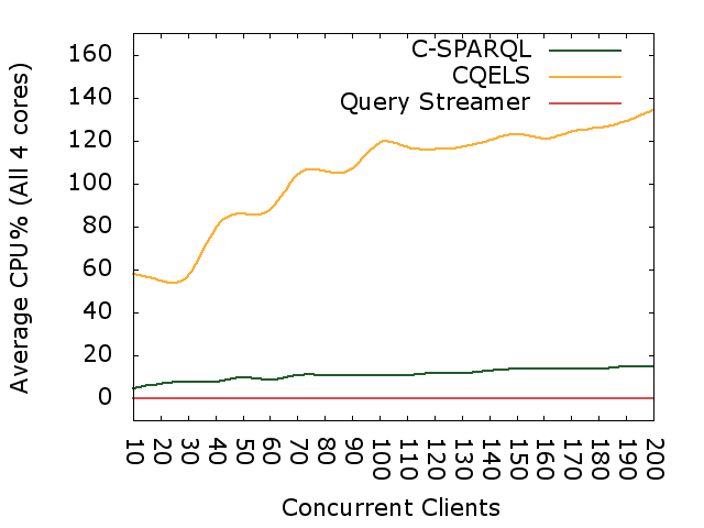
Subfig. 42.1: The server CPU usage of our solution proves to be influenced less by the number of clients.
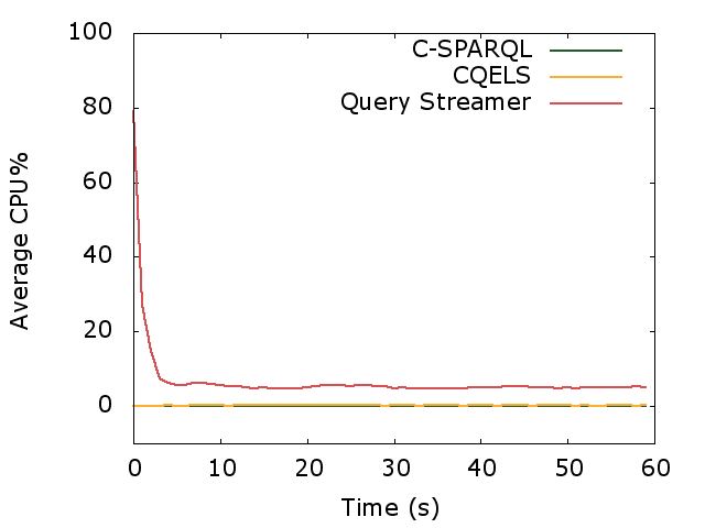
Subfig. 42.2: In the case of 200 concurrent clients, client CPU usage initially is high after which it converges to about 5%. The usage for C-SPARQL and CQELS is almost non-existing.
Fig. 42: Average server and client CPU usage for one query stream for C-SPARQL, CQELS and the proposed solution. Our solution effectively moves complexity from the server to the client.
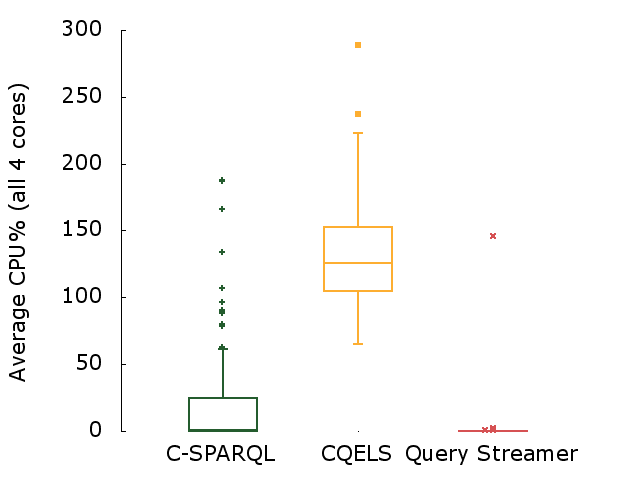
Subfig. 43.1: Server CPU peaks for C-SPARQL and CQELS compared to our solution.
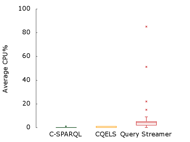
Subfig. 43.2: Client CPU usage for our solution is significantly higher.
Fig. 43: Detailed view on all server and client CPU measurements for C-SPARQL, CQELS and the solution presented in this work for 200 simultaneous query evaluations against the server.
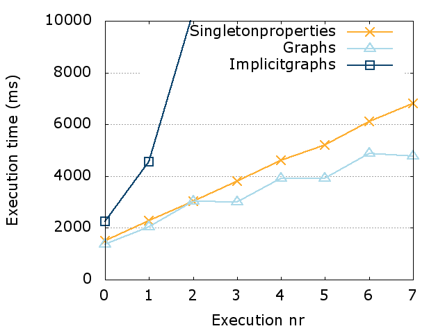
Subfig. 44.1: Time intervals without caching.
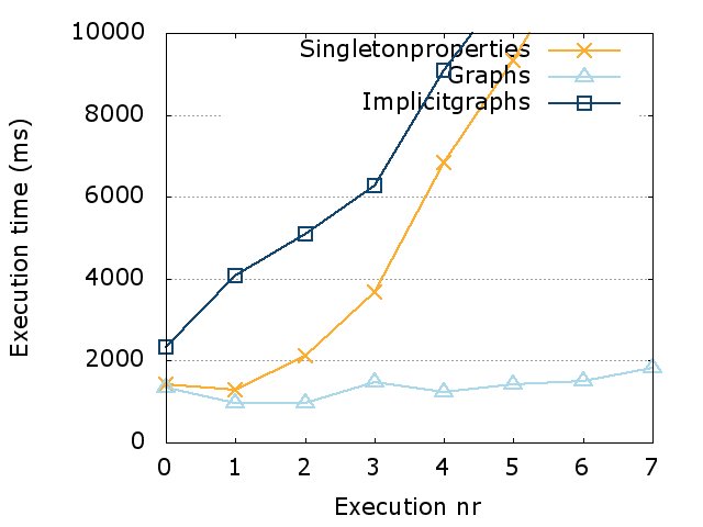
Subfig. 44.2: Time intervals with caching.
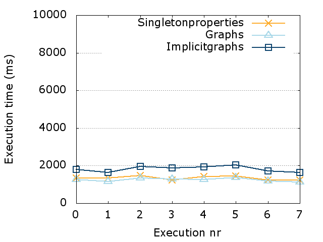
Subfig. 44.3: Expiration times without caching.
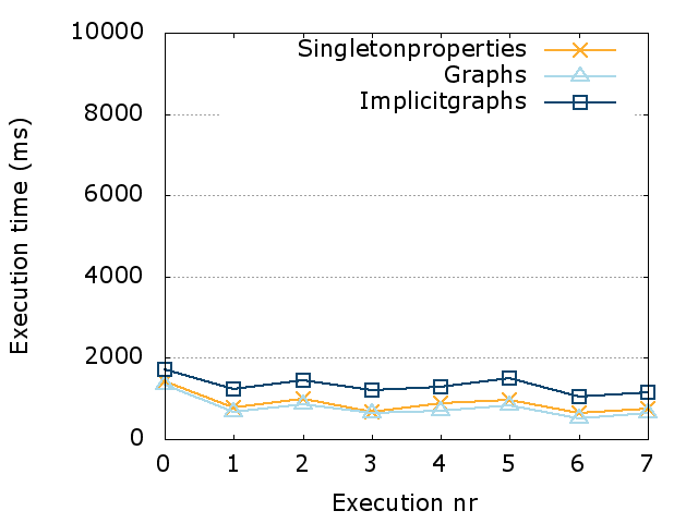
Subfig. 44.4: Expiration times with caching.
Fig. 44: Executions times for the three different types of dynamic data representation for several subsequent streaming requests. The figures show a mostly linear increase when using time intervals and constant execution times for annotation using expiration times. In general, caching results in lower execution times. They also reveal that the graph approach has the lowest execution times.
Conclusions
In this paper, we researched a solution for querying over dynamic data with a low server cost, by continuously polling the data based on volatility information. In this section, we draw conclusions from our evaluation results to give an answer to the research questions and hypotheses we defined in Section 5.3. First, the server and client costs for our solution will be compared with the alternatives. After that, the effect of our client-side cache will be explained. Next, we will discuss the effect of time annotation on the amount of requests to be sent, after which the performance of our solution will be shown and the effects of the annotation methods.
Server cost
The results from Subsection 5.7.1 confirm Hypothesis 1, in which we wanted to know if we could lower the server cost when compared to C-SPARQL and CQELS. Not only is the server cost for our solution more than ten times lower on average when compared to the alternatives, this cost also increases much slower for a growing number of simultaneous clients. This makes our proposed solution more scalable for the server. Another disadvantage of C-SPARQL and CQELS is the fact that the server load for a large number of concurrent clients varies significantly, as can be seen in Subfig. 43.1. This makes it hard to scale the required processing powers for servers using these technologies. Our solution has a low and more constant CPU usage.
Client cost
The results for the client load measurements from Subsection 5.7.2 confirm Hypothesis 2, which stated that our solution increases the client’s processing need. The required client processing power using our solution is clearly much higher than for C-SPARQL and CQELS. This is because we redistributed the required processing power from the server to the client. In our solution, it is the client that has to do most of the work for evaluating queries, which puts less load on the server. The load on the client still remains around 5% for the largest part of the query evaluation as shown in Subfig. 42.2. Only during the first few seconds, the query engines CPU usage peaks, which is because of the processor-intensive rewriting step that needs to be done once at the start of each dynamic query evaluation.
Caching
We can also confirm Hypothesis 3 about the positive effect of caching from the results in Subsection 5.7.3. Our caching solution has a positive effect on the execution times. In an optimal scenario for our use case, caching would lead to an execution time reduction of 60% because three of the five triple patterns in the query for our use case from Section 5.4 are static. For our results, this caching leads to an average reduction of 56% which is close to the optimal case. Since we are working with dynamic data, some required background-data is bound to overlap, in these cases it is advantageous to have a client-side caching solution so that these redundant requests for static data can be avoided. The longer our query evaluation runs, the more static data the cache accumulates, so the bigger the chance that there are cache hits when background data is needed in a certain query iteration. Future research should indicate what the limits of such a client-side cache for static data are, and whether or not it is advantageous to reuse this cache for different queries.
Request reduction
By annotating dynamic data with a time annotation, we successfully reduced the amount of required requests for polling-based SPARQL querying to a minimum, which answers Research Question 1 about the question if clients can use volatility knowledge to perform continuous querying. Because now, the client can derive the exact moment at which the data can change on the server, and this will be used to schedule a new query execution on the server. In future research, it is still possible to reduce the amount of requests our client engine needs to send through a better caching strategy, which could for example also temporarily cache dynamic data which changes at different frequencies. We can also look into differential data transmission by only sending data to the client that has been changed since the last time the client has requested a specific resource.
Performance
For answering Research Question 2, the performance of our solution compared to alternatives, we compared our solution with two state-of-the-art approaches for dynamic SPARQL querying. Our solution significantly reduces the required server processing per client, this complexity is mostly moved to the client. This comparison shows that our technique allows data providers to offer dynamic data which can be used to continuously evaluate dynamic queries with a low server cost. Our low-cost publication technique for dynamic data is useful when the number of potential simultaneous clients is large. When this data is needed for only a small number of clients in a closed off environment and query evaluation must happen fast, traditional approaches like CQELS or C-SPARQL are advised. These are only two possible points on the Linked Data Fragments axis [36], depending on the publication requirements, combinations of these approaches can be used.
Annotation methods
In Research Question 3, we wanted to know how the different annotation methods influenced the execution times. From the results in Subsection 5.7.3, we can conclude that graph-based annotation results in the lowest execution times. It can also be seen that annotation with time intervals has the problem of continuously increasing execution times, because of the continuously growing dataset. Time interval annotation can be desired if we for example want to maintain the history of certain facts, as opposed to just having the last version of facts using expiration times. In future work, we will investigate alternative techniques to support time interval annotation without the continuously increasing execution times.
In this work, the frequency at which our queries are updated is purely data-driven using time intervals or expiration times. In the future it might be interesting, to provide a control to the user to change this frequency, if for example this user only desires query updates at a lower frequency than the data actually changes.
In future work, it is important to test this approach with a larger variety of use cases. The time annotation mechanisms we use are generic enough to transform all static facts to dynamic data for any number of triples. The CityBench [34] benchmark can for example be used to evaluate these different cases based on city sensor data. These tests must be scaled (both in terms of clients as in terms of dataset size), so that the maximum number of concurrent requests can be determined, with respect to the dataset size.
Addendum
In this section, I summarize the follow-up work that has been done since the article corresponding to this chapter has been published. Concretely, I focus on “On the Semantics of TPF-QS towards Publishing and Querying RDF Streams at Web-scale” [129] that has been published two years after the work from this chapter. This article aims to resolve some of the initial weaknesses. Concretely, a proper formalization is introduced, using which the system (TPF-QS) is compared using alternative RDF stream processing systems. Furthermore, a more extensive evaluation is done using a state of the art benchmark. These two parts are summarized hereafter.
Formalization
RSP-QL [130] is a formal reference model in which different RDF Stream Processing (RSP) systems can be compared to each other, such as C-SPARQL [15], CQELS [16] and TPF-QS [96]. It can be seen as an extension of RDF and SPARQL, by introducing temporal semantics. In the next paragraphs, I will summarize the RSP-QL model, explain how TPF-QS fits into this, and how TPF-QS can be compared to alternative RSP systems using this model. I will omit the details and full formal definitions that can be found in the full paper [129].
RSP-QL Overview
RSP-QL introduces the concept of an RDF stream that is defined as an unbounded sequence of pairs. Each pair consists of an RDF statement and a time instant.
In order to query RDF streams, the concept of an RDF dataset was extended to an RSP-QL dataset. Such a dataset consists of an optional default graph, zero or more named graphs, and zero or more (named) time-varying graphs. A time-varying graph is a function that maps time instants to instantaneous RDF graphs.
To avoid querying over very large streams, the concept of a time-based window was introduced. A time-based window is defined by a certain width, a slide parameter, and a starting time, where all of these parameters are expressed in time units. Concretely, such a window takes an RDF stream as input, and produces a time-varying graph.
To model the different ways in which repeated query evaluation can occur, so-called evaluation strategies were introduced. For example, the Content Change (CC) strategy makes the window report results when window contents change. Window Close (WC) reports when the window closes. The Non-empty Content (NC) strategy reports if the active window is not empty. The Periodic (P) stategy reports at regular time intervals.
Finally, after windowing, query execution results can be reported in different ways, where each of them adds time annotations to the solution mappings. RStream annotates an input sequence of solution mappings with the evaluation time; IStream streams the difference between the answer of the current evaluation and the one of the previous iteration; DStream streams the part of the answer at the previous iteration that is not in the current one.
TPF-QS in terms of RSP-QL
From the perspective of a TPF-QS client, the data that was retrieved from a TPF server can be interpreted as an RSP-QL stream, for which we introduced a formal mapping. Based on this, all elements of the RSP-QL model can be applied.
Windows within TPF-QS can have a configurable starting time, and always have a width and slide parameter of exactly one time unit. As a consequence, the evaluation of a window in TPF-QS will always produce a time-varying graph that contains exactly one instantaneous RDF graph.
TPF-QS supports two configurable evaluation strategies: Periodic and Mapping Expire (ME). The Mapping Expire strategy is specific to TPF-QS, and is possible because of the time validity annotations that are exposed by TPF servers. In summary, Mapping Expire will make the window report when the validity of an RDF statement that was used in the last solution mapping expires.
RSP-QL Comparison
Table 16 compares the TPF-QS with C-SPARQL and CQELS in terms of the RSP-QL reference model.
| Feature | TPF-QS | C-SPARQL | CQELS |
|---|---|---|---|
| volatile RDF stream | no | yes | yes |
| data retrieval | pull | push | push |
| time annotation | time interval | timestamp | timestamp |
| window parameters | configurable starting time, width and slide of one time unit | fixed starting time, configurable width and slide | fixed starting time, configurable width and slide |
| RSP-QL dataset | time varying graph in default graph | time varying graph in default graph | named time varying graph |
| window policy | ME, P | WC, NC | CC |
| streaming operators | RStream | RStream | IStream |
Table 16: Comparison TPF-QS, C-SPARQL, and CQELS in terms of the main elements of the RSP-QL reference model.
Evaluation
While the experiments that were presented in this chapter made use of a relatively small dataset with simple queries, our new experiments made use of the CityBench [34] benchmark. Using this benchmark, large-scale real-world sensor data streams were used together with a set of realistic queries, ranging from simple to complex. For an increasing number of clients, we measured server CPU usage, result latency, result completeness. Using CityBench, we compared TPF-QS with C-SPARQL and CQELS. Our findings show that TPF-QS results in lower server load and latency for simple queries, but higher for complex queries. Due to slower evaluation, TPF-QS sometimes results in lower result completeness than the alternatives.
Results clearly show that when stream volatility is constant, and queries are not too complex, TPF-QS outperforms alternative systems in terms of server load for an increasing number of clients. However, there is still a limit in the number of concurrent clients that can be achieved, since the results have shown that result latencies start increasing for high numbers of clients. This shows that TPF-QS should only be used in specific use cases, and that additional follow-up work is required to make it more widely applicable.
Conclusions
The research question of this PhD was defined as “How to store and query evolving knowledge graphs on the Web?” The answer to this question is neither simple nor complete. In this final chapter, I first summarize an answer to this question, the limitations of my work, and I discuss future research efforts that are needed to advance this work further.
Contributions
Based on my research question, I focussed on four main challenges:
- Experimentation requires representative evolving data.
- Indexing evolving data involves a trade-off between storage efficiency and lookup efficiency.
- Web interfaces are highly heterogeneous.
- Publishing evolving data via a queryable interface involves continuous updates to clients.
I will discuss the findings within these challenges hereafter.
Generating Evolving Data
In Chapter 2, the first challenge was tackled as a prerequisite for the next challenges. The domain of public transport was chosen for this challenge, as it contains both geospatial and temporal dimensions, which makes it useful for benchmarking RDF data management systems that can handle various dimensions like these. Even though many real-world public transit network design and scheduling methodologies already exist, the synthetic generation of such datasets is not trivial. The goal of this work was to determine wether or not population distributions could be used as input to such a mimicking algorithm. Hence, this lead to the following research question:
Can population distribution data be used to generate realistic synthetic public transport networks and scheduling?
The main hypothesis of this work was: public transport networks and schedules are correlated with the population distribution within the same area. This hypothesis was tested and validated for two countries with a high level of confidence. As such, population distributions formed the basis of the mimicking algorithm of this work.
Inspired by real-world public transit network design and scheduling methodologies, a multi-step algorithm was determined where regions, stops, edges, routes and trips are generated based on any population distribution and dependency rules. To evaluate the realism of generated datasets, an implementation of the algorithm was provided. For each step in the algorithm, distance functions were determined to measure the realism for each step. This realism was confirmed for different regions and transport types.
With the provided mimicking algorithm, synthetic public transport networks and scheduling can be generated based on population distributions, which answers our research question. This tackles our initial challenge to support experimentation on systems that handle evolving knowledge graphs.
Indexing Evolving Data
Next, in Chapter 3, the challenge was to determine an approach that achieves a trade-off between storage size and lookup efficiency that is beneficial for publishing evolving knowledge graphs on the Web. This approach had to enable a Web-friendly storage approach, so that evolving knowledge graphs can be published on the Web without requiring very costly machines. Previous work has shown that by restricting queries on servers to triple pattern queries [36], and executing more complex queries client-side, server load can be reduced significantly. As such, our work built upon this idea by focusing on triple pattern queries. Furthermore, to reduce memory usage during query execution, we focus on streaming results with optional offsets. Finally, we focus on three main versioned query atoms to support various kinds of temporal queries over evolving knowledge graphs. This lead to the following research question:
How can we store RDF archives to enable efficient versioned triple pattern queries with offsets?
This research question is answered by introducing (1) a storage technique for maintaining multiple versions of a knowledge graph and (2) querying algorithms that can be used to efficiently extract data from these versions. As was shown via our hypotheses, this storage technique is a hybrid of different existing storage approaches, which lead to a trade-off between all of them in terms of storage requirements and querying efficiency. Important to note is that the introduced storage technique is therefore not the most optimal for all situations. For specific use cases where only very specific query types are required, dedicated systems will likely be more efficient. However, when the domain of queries is broad, a more general-purpose like our approach is more fitting, as this will lead to sufficiently fast query execution in most cases, with acceptable storage requirements.
In conclusion, our storage approach can be used be used as a backend for publishing evolving knowledge graphs through a low-cost triple pattern interface, which has been illustrated via Versioned Triple Pattern Fragments [42] on http://versioned.linkeddatafragments.org/bear. Future challenges include the handling of very large numbers of versions and improving ingestion efficiency, which both could be resolved by dynamically creating intermediary snapshots within the delta chain.
Heterogeneous Web Interfaces
In Chapter 4, the challenge on handling the heterogeneous nature of Web interfaces during querying was tackled. This was done through the design and development of a highly modular meta query engine (Comunica) that simplifies the handling of various kinds of sources, and lowers the barrier for researching new query interfaces and algorithms.
In order for Comunica to be usable as a research platform, its architecture needed to be flexible enough to handle the complete SPARQL 1.1 specification, and support heterogeneous interfaces. For this, the actor, mediator, and publish-subscribe software patterns were applied to achieve an architecture where task-specific actors form building blocks, and buses and mediators are used to handle their inter-communication, which can be wired together through dependency injection.
With Comunica, evaluating the performance of different query algorithms and other query-related approaches become more fair. Query algorithms are typically compared by implementing them in separate systems, which leads to confounding factors that may impact the performance results, such as the use of different programming languages or software libraries. As Comunica consists of small task-specific building blocks, different algorithms become different instances of such building blocks, which reduces confounding during experiments.
Comunica’s architecture is flexible enough to go outside the realm of standard SPARQL. It is for example usable to create an engine for querying over evolving knowledge graphs [131]. Concretely, support for OSTRICH datasources from Chapter 3 was implemented, together with support for versioned queries. For this, the streaming results capability of OSTRICH proved compatible and beneficial to the streaming query evaluation of Comunica.
Publishing and Querying Evolving Data
Finally, Chapter 5 handled the challenge on a query interface for evolving knowledge graphs. The main goal of this work was to determine whether (part of) the effort for executing continuous queries over evolving knowledge graphs could be moved from server to client, in order to allow the server to handle more concurrent clients. The outcome of this work was a polling-based Web interface for evolving knowledge graphs, and a client-side algorithm that is able to perform continuous queries using this interface.
The first research question of this work was:
Can clients use volatility knowledge to perform more efficient continuous SPARQL query evaluation by polling for data?
This question was answered by annotating dynamic data server-side with time annotations, and by introducing a client-side algorithm that can detect these annotations, and determine a polling frequency for continuous query evaluation based on that. By doing this, clients only have to re-download data from the server when it was changed. Furthermore, static data only have to be downloaded once from the server when needed, and can therefore optimally be cached by the client. In practise, one could however argue that no data is never truly indefinitely static, which is why practical implementations will require caches with a high maximum age for static data when performing continuous querying over long periods of time.
Our second research question was formulated as:
How does the client and server load of our solution compare to alternatives?
This question was answered by comparing the server and client load of our approach with state of the art server-side engines. Results show a clear movement of load from server to client, at the cost of increased bandwidth usage and execution time. The benefit of this becomes especially clear when the number of concurrent clients increase. The server load of our approach scales significantly better compared to other approaches for an increasing number of clients. This is caused by the fact that each clients now helps with query execution, which frees up a significant portion of server load. Since multiple concurrent clients also lead to server requests for overlapping URLs, a server cache should theoretically be beneficial as well. However, follow-up work has shown that such a cache leads to higher server load [129] due to the high cost of cache invalidation over dynamic data. This shows that caching dynamic data is unlikely to achieve overall performance benefits. More intelligent caching techniques may lead to better efficiency, by for example only caching data that will be valid for at least a given time period.
The final research question was defined as:
How do different time-annotation methods perform in terms of the resulting execution times?
Results have shown that by exploiting named graphs for annotating expiration times to dynamic data, total execution times are the lowest compared to other annotation approaches. This is caused by the fact that the named graphs approach leads to a lower amount of triples to be downloaded from the server. And since bandwidth usage has a significant impact on query execution times, the number of triples that need to be download have such an impact.
Overview
By investigating these four challenges, our main research question can be answered. Concretely, evolving knowledge graphs with a low volatility (order of minutes or slower) can be made queryable on the Web through a low-cost polling-based interface, with a hybrid snapshot/delta/timestamp-based storage system in the back end. On top of this and other interfaces, intelligent client-side query engines can perform continuous queries. This comes at the cost of an increase in bandwidth usage and execution time, but with a higher guarantee on result completeness as server availability is improved. All of this can be evaluated thoroughly using synthetic evolving datasets that can for example be generated with a mimicking algorithm for public transport network.
This proves that evolving knowledge graphs can be published and queried on the Web. Furthermore, no high-cost Web infrastructure is needed to publish or query such graphs, which lowers the barrier for smaller, decentralized evolving knowledge graphs to be published, without having to be a giant company with a large budget.
Limitations
There are several limitations to my contributions that require attention, which will be discussed hereafter.
Generating Evolving Data
In Chapter 2, I introduced a mimicking algorithm for generating public transport datasets. One could however question whether such domain-specific datasets are sufficient for testing evolving knowledge graphs systems in general. As shown in Section 2.5, the introduced data model contains a relatively small number of RDF properties and classes. While large domain specific knowledge graphs like these are valuable, domain-overlapping knowledge graphs such as DBpedia [40] and Wikidata [132] many more distinct properties and classes, which place additional demands on systems. For such cases, multi-domain (evolving) knowledge graph generators could be created in future work.
Furthermore, the mimicking algorithm produces temporal data in a batch-based manner, instead of a continuous streaming process. This requires an evolving knowledge graph to be produced with a fixed temporal range, and does it does not allow knowledge graphs to evolve continuously for an non-predetermined amount of time. The latter would be valuable for stream processing systems that need to be evaluated for long periods of time, which would require an adaptation to the algorithm to make it streaming.
Indexing Evolving Data
In Chapter 3, a storage mechanism for evolving knowledge graphs was introduced. The main limitation of this work is that ingestion times continuously increase when more versions are added. This is caused by the fact that versions are typically relative to the previous version, whereas this storage approach handles versions relative to the initial version. As such, such versions need to be converted at ingestion time, which takes continuously longer for more versions. This shows that this approach can currently not be used for knowledge graphs that evolve indefinitely long, such as DBpedia Live [78]. One possible solution to this problem would be to fully maintain the latest version for faster relative version recalculation.
The second main limitation is the fact that delta (DM) queries do not efficiently support result offsets. As such, my approach is not ideal for use cases where random-access in version differences is needed within very large evolving knowledge graphs, such as for example finding the 10th or 1000th most read book between 2018 and 2019. My algorithm naively applies an offset by iterating and voiding results until the offset amount is reach, as opposed to the more intelligent offset algorithms for the other versioned query types where an index is used to apply the offset. One possible solution would be to add an additional index for optimizing the offsets for delta queries, which would also lead to increased storage space and ingestion times.
Heterogeneous Web Interfaces
The main limitation of the Comunica meta query engine from Chapter 4 is its non-interruptible architecture. This means that once the execution of a certain query operation is started, it can not be stopped until it is completed without killing the engine completely. This means that meta-algorithms that dynamically switch between algorithms depending on their execution times can not be implemented within Comunica. In order to make this possible, a significant change to the architecture of Comunica would be required where every actor could be interrupted after being started, where these interruptions would have to be propagated through to chained operations.
Another limitation of Comunica is its development complexity, which is a consequence of its modularity. Practise has shown that there is a steep learning curve for adding new modules to Comunica, which is due to the dependency injection system that is error-prone. To alleviate this problem, tutorials are being created and presented, and tools are being developed to simplify the usage of the dependency injection framework. Furthermore, higher-level tools such as GraphQL-LD [133] and LDflex are being developed to lower the barrier for querying with Comunica.
Publishing and Querying Evolving Data
The main limitation of our publishing and querying approach for evolving data from Chapter 5 is the fact that it only works for slowly evolving data. From the moment that data changes at the order of one second or faster, then the polling-based query approach becomes too slow, and results become outdated even before they are produced. This is mainly caused by the roundtrip times of HTTP requests, and the fact that multiple of them are needed because of the Triple Pattern Fragments querying approach. For data that evolves much faster, a polling-based approach like this is not a good solution. Socket-like solutions where client and server maintain an open connection would be able to reach much higher data velocities, since servers can send updates to subscribed clients immediately, without having to wait for a client request, which reduces result latency.
The second limitation to consider is the significantly higher bandwidth usage compared to other approaches, which has been shown in follow-up work [129]. This means that this approach is not ideal for use cases where bandwidth is limited, such as querying from low-end mobile devices, or querying in rural areas with a slow internet connection. This higher bandwidth usage is inherent to the Triple Pattern Fragments approach, since more data needs to be downloaded from the server, so that the client can process it locally.
Open Challenges
While I have formulated one possible answer the question on how to store and query evolving knowledge graphs on the Web, this is definitely not the only answer. As such, further research is needed on all aspects.
Regarding the storage aspect, alternative techniques for storing evolving knowledge graphs with different trade-offs will be useful for different scenarios. On the one hand, dedicated storage techniques should be developed for low-end devices, such as small sensors in the Internet of Things. On the other hand, storage techniques should be developed for very high-end devices, such as required for the infrastructure within nuclear reactors.
Furthermore, current storage solutions mainly focus on the syntactical querying over evolving knowledge graphs, but they do not really consider the issue of semantic querying [134] yet, which involves taking into account the meaning of things through ontology-based inferencing. Semantic querying over evolving knowledge graphs is needed to enable semantic analysis over such knowledge, such as analyzing concept drift [135] or tracking diseases in biomedical datasets over time [136]. As such, the area of semantic querying over evolving knowledge graphs requires further research.
During this PhD, I mainly focused on publishing and querying evolving knowledge graphs with predictable periodicity in the order of one minute. Knowledge graphs with faster, slower or unpredictable periodicities may require different techniques. As such, more work is needed to investigate the impact of different kinds of evolving knowledge graphs on publishing and querying. For instance, evolving knowledge graphs with slower periodicities may benefit more from being published through an interface that is well cacheable, compared to more volatile knowledge graphs.
Next, standardization efforts will be needed to truly bring evolving knowledge graphs to the Web, in the form of temporal query languages, temporal models and exchange formats. For the sake of compatibility, these should be extensions or they should be representable in the existing Linked Data stack, which will mainly impact RDF and SPARQL. The W3C RDF Stream Processing community group is a first effort that aims to explore these issues.
Due to the many remaining challenges, it will take more research and engineering effort before we will see the true adoption of publishing and querying evolving knowledge graphs on the Web. Nevertheless, it is important to open up these evolving knowledge graphs to the public Web, so that humanity can benefit from this as whole, instead of only being usable by organizations internally behind closed doors.
In a broader sense, more work will be needed to solve open problems with decentralized knowledge graphs. The Solid ecosystem [137] is becoming an important driver within this decentralization effort, as it offers several fundamental standards to build a decentralized Web. As such, future Web research will benefit significantly by building upon these standards. Concretely, new techniques and algorithms are needed to (1) intelligently navigate the the Web by following relevant links for a given query [89], (2) enable efficient querying over a large number of sources, (3) allow authentication-aware querying over private data, and (4) support collaborative querying between agents that handle similar queries.
Next to these technical issues, organizational and societal changes will also be needed. For instance, the European General Data Protection Regulation places strict demands on companies that handle personal data. Decentralization efforts such as Solid are being investigated by organizations such as governments to reshape the relationship with their citizens [138], by giving people true ownership over their data, and making governments data consumers.
As I placed a strong emphasis on reusability during this PhD, all of the tools and experiments that were implemented are available under an open license. Furthermore, well-established development methods from the software industry were followed to achieve implementations with decent code quality and valuable usage and development documentation. This should therefore lower the barrier for other researchers in the future to build upon this research and its tools.
For the next couple of years, I aim to focus more on the topic of querying decentralized knowledge graphs. For this, I will collaborate further with my colleagues from IDLab, researchers from other labs, and companies with similar goals. With this, I hope to empower individuals on the Web, by allowing them to find the information they want, instead of what is being forced upon them, which is a fundamental human right.